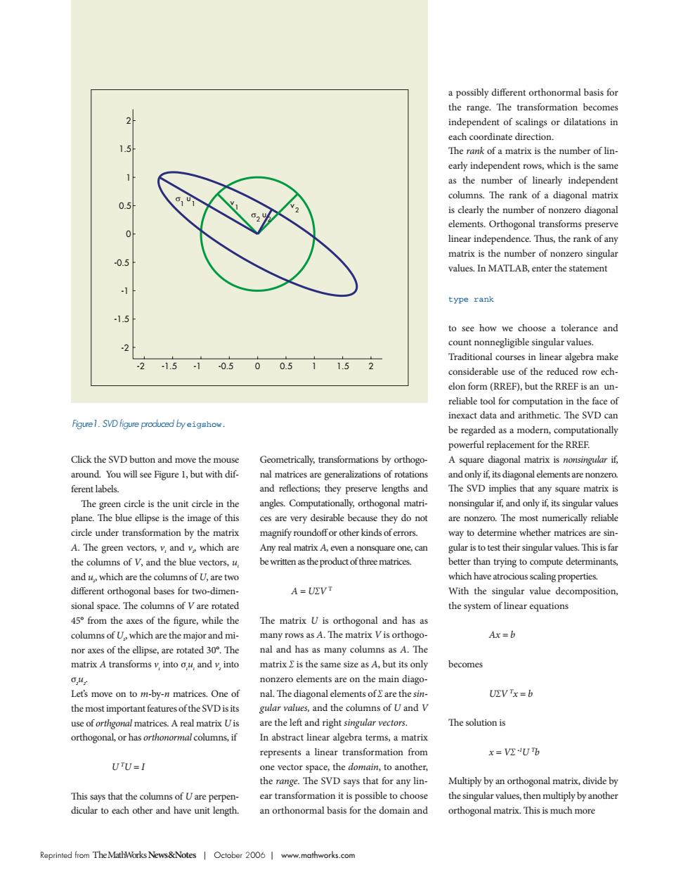
on b indene dent of scalings or dilatations in each coordinate direction 1.5 The rank of a matrix is the number of lin early independent rows.which is the same as the number of linearly independen columns.The rank of a diagonal matrix 0.5 s clearly the number of nonzero diagonal elements.Orthogonal type rank 15 tole eand hra make 050051152 elon form (rrer but the rreeis an un reliable tool for computation in the face of inexact data and arithmetic.The SyD can gre.SVDfigure prodced byghw be regarded as a modern,computationally powerful replacement for the RREF Click the SVD button and move the mouse Geometrically,transformations by orthogo- A square diagonal matrix is nonsingular if around.You will see Figure 1,but with dif. erent labels. eflections;they pre rve lengths SVD imple any square m灯 y,orthogonal i道iss pse is the re very other kind are no of V and the ki e roduct of three different orthoa nalbases for two-dime A=UVT sional space The columns of y are motated the system of linear quations 45 from the axes of the figure while the The matrix U is orthogonal and has as columns of U.which are the major and mi- many rows as A.The matrix Vis orthogo Ax=b nor axes of the ellipse,are rotated 30".The nal and has as many columns as A.The matrix A transforms v.into ou and v.into matrix 2 is the same size as A,but its only becomes nonzero elements are on the main diago on to m-by-matrices.One of nal.The diagonal elements of 2 are the si =b the most important features ofthe SVDist valles,and the mns of U and v mat re the lent and ngh atri x=U any lin Multiply by an orthogonal matrix.divide by sible to ch an orthonormal basis for the domain and Reprinted from The MathWorks News&Notes Oclober 2006 www.mathworks.comReprinted from T heMathWorksNews&Notes | October 2006 | www.mathworks.com Click the SVD button and move the mouse around. You will see Figure 1, but with dif￾ferent labels. The green circle is the unit circle in the plane. The blue ellipse is the image of this circle under transformation by the matrix A. The green vectors, v1 and v2 , which are the columns of V, and the blue vectors, u1 and u2 , which are the columns of U, are two different orthogonal bases for two-dimen￾sional space. The columns of V are rotated 45° from the axes of the figure, while the columns of U2 , which are the major and mi￾nor axes of the ellipse, are rotated 30°. The matrix A transforms v1 into σ1 u1 and v2 into σ2 u2 . Let’s move on to m-by-n matrices. One of the most important features of the SVD is its use of orthgonal matrices. A real matrix U is orthogonal, or has orthonormal columns, if U TU = I This says that the columns of U are perpen￾dicular to each other and have unit length. Geometrically, transformations by orthogo￾nal matrices are generalizations of rotations and reflections; they preserve lengths and angles. Computationally, orthogonal matri￾ces are very desirable because they do not magnify roundoff or other kinds of errors. Any real matrix A, even a nonsquare one, can be written as the product of three matrices. A = U∑V T The matrix U is orthogonal and has as many rows as A. The matrix V is orthogo￾nal and has as many columns as A. The matrix ∑ is the same size as A, but its only nonzero elements are on the main diago￾nal. The diagonal elements of ∑ are the sin￾gular values, and the columns of U and V are the left and right singular vectors. In abstract linear algebra terms, a matrix represents a linear transformation from one vector space, the domain, to another, the range. The SVD says that for any lin￾ear transformation it is possible to choose an orthonormal basis for the domain and a possibly different orthonormal basis for the range. The transformation becomes independent of scalings or dilatations in each coordinate direction. The rank of a matrix is the number of lin￾early independent rows, which is the same as the number of linearly independent columns. The rank of a diagonal matrix is clearly the number of nonzero diagonal elements. Orthogonal transforms preserve linear independence. Thus, the rank of any matrix is the number of nonzero singular values. In MATLAB, enter the statement type rank to see how we choose a tolerance and count nonnegligible singular values. Traditional courses in linear algebra make considerable use of the reduced row ech￾elon form (RREF), but the RREF is an un￾reliable tool for computation in the face of inexact data and arithmetic. The SVD can be regarded as a modern, computationally powerful replacement for the RREF. A square diagonal matrix is nonsingular if, and only if, its diagonal elements are nonzero. The SVD implies that any square matrix is nonsingular if, and only if, its singular values are nonzero. The most numerically reliable way to determine whether matrices are sin￾gular is to test their singular values. This is far better than trying to compute determinants, which have atrocious scaling properties. With the singular value decomposition, the system of linear equations Ax = b becomes U∑V Tx = b The solution is x = V∑ -1U Tb Multiply by an orthogonal matrix, divide by the singular values, then multiply by another orthogonal matrix. This is much more -2 -1.5 -1 -0.5 0 0.5 1 1.5 2 -2 -1.5 -1 -0.5 0 0.5 1 1.5 2 v 1 v 2 σ1 u1 σ2 u2 Figure1. SVD figure produced by eigshow