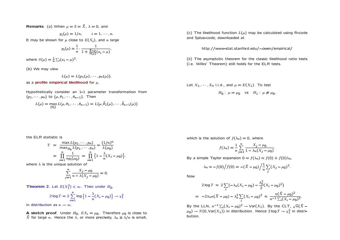
Remarks.(a)When===0,and p:(m）=1/mi=1,…,n. (c)The likelihood function L()may be calculated using R-code It may be shown for u close to E(X;).and n large and Splus-code,downloaded at n0片1+新e-可 1 http://www-stat.stanford.edu/~owen/empirical/ where S(w)=∑：(ri-r)2. (ii)The asymptotic theorem for the classic likelihood ratio tests (i.e.Wilks'Theorem)still holds for the ELR tests. (b)We may view L()=L{p1(r),…,p()} as a profile empirical likelihood for u. Let X1,.…,Xni.i.d.,andμ=E(Xi).To test Hypothetically consider an 1-1 parameter transformation from H0:μ=0vsH1:μ≠0： {p1,…,pm}to{u,01,…,0m-1}.Then L()=maxL(4,01,…,0n-1)=L{4,01(μ），…，0n-1(4)} {} the ELR statistic is which is the solution of f(An)=0,where T max L(p1,....pn)(1/n)" maxH L(p1,…,P)=io (n)= ，X-0 n台11-n(Xy-o) inp(o)s】 红-acx-o以 =1 By a simple Taylor expansion 0=f(An)f(0)+f(0)An, where A is the unique solution of X-40 g-o/io)=-(-o/月x-o2 含-o =0 Now Theorem 2.Let E(X)<oo.Then under Ho. 2gTs2罗--o)-当0x-o月 21ogT=21og{1-2x-o)}一x好 =-2nn(R-4o)-2∑(X-Ho2≈n-2x-o2 n(灭-4o)2 =1 in distribution as n-oo. By the LLN,n-1∑(Xi-μo)2→Var(Xi).By the CLT,vm(r- A sketch proof.Under Ho.EX;=Ho.Therefore Ho is close to Ho)-N(0,Var(X1))in distribution.Hence 2 log Tx in distri- Xfor large n.Hence the )or more precisely.n =A/n is small, bution.Remarks. (a) When µ = ¯x = X¯, λ = 0, and pi(µ) = 1/n, i = 1, · · · , n. It may be shown for µ close to E(Xi), and n large pi(µ) ≈ 1 n · 1 1 + x¯−µ S(µ) (xi − µ) , where S(µ) = 1 n P i(xi − µ) 2. (b) We may view L(µ) = L{p1(µ), · · · , pn(µ)}. as a profile empirical likelihood for µ. Hypothetically consider an 1-1 parameter transformation from {p1, · · · , pn} to {µ, θ1, · · · , θn−1}. Then L(µ) = max {θi} L(µ, θ1, · · · , θn−1) = L{µ, bθ1(µ), · · · , bθn−1(µ)} (c) The likelihood function L(µ) may be calculated using R-code and Splus-code, downloaded at http://www-stat.stanford.edu/∼owen/empirical/ (ii) The asymptotic theorem for the classic likelihood ratio tests (i.e. Wilks’ Theorem) still holds for the ELR tests. Let X1, · · · , Xn i.i.d., and µ = E(X1). To test H0 : µ = µ0 vs H1 : µ 6= µ0, the ELR statistic is T = max L(p1, · · · , pn) maxH0 L(p1, · · · , pn) = (1/n) n L(µ0) = Yn i=1 1 npi(µ0) = Yn i=1 n 1 − λ n (Xi − µ0) o . where λ is the unique solution of Xn j=1 Xj − µ0 n − λ(Xj − µ0) = 0. Theorem 2. Let E(X2 1 ) < ∞. Then under H0, 2 log T = 2 Xn i=1 log n 1 − λ n (Xi − µ0) o → χ 2 1 in distribution as n → ∞. A sketch proof. Under H0, EXi = µ0. Therefore µ0 is close to X¯ for large n. Hence the λ, or more precisely, λn ≡ λ/n is small, which is the solution of f(λn) = 0, where f(λn) = 1 n Xn j=1 Xj − µ0 1 − λn(Xj − µ0) . By a simple Taylor expansion 0 = f(λn) ≈ f(0) + f˙(0)λn, λn ≈ −f(0). f˙(0) = −(X¯ − µ0) 1 n X j (Xj − µ0) 2 . Now 2 log T ≈ 2 X i {−λn(Xi − µ0) − λ 2 n 2 (Xi − µ0) 2 } = −2λnn(X¯ − µ0) − λ 2 n X i (Xi − µ0) 2 ≈ n(X¯ − µ0) 2 n−1 P i(Xi − µ0) 2 . By the LLN, n −1 P i(Xi − µ0) 2 → Var(X1). By the CLT, √ n(X¯ − µ0) → N(0, Var(X1)) in distribution. Hence 2 log T → χ 2 1 in distri￾bution