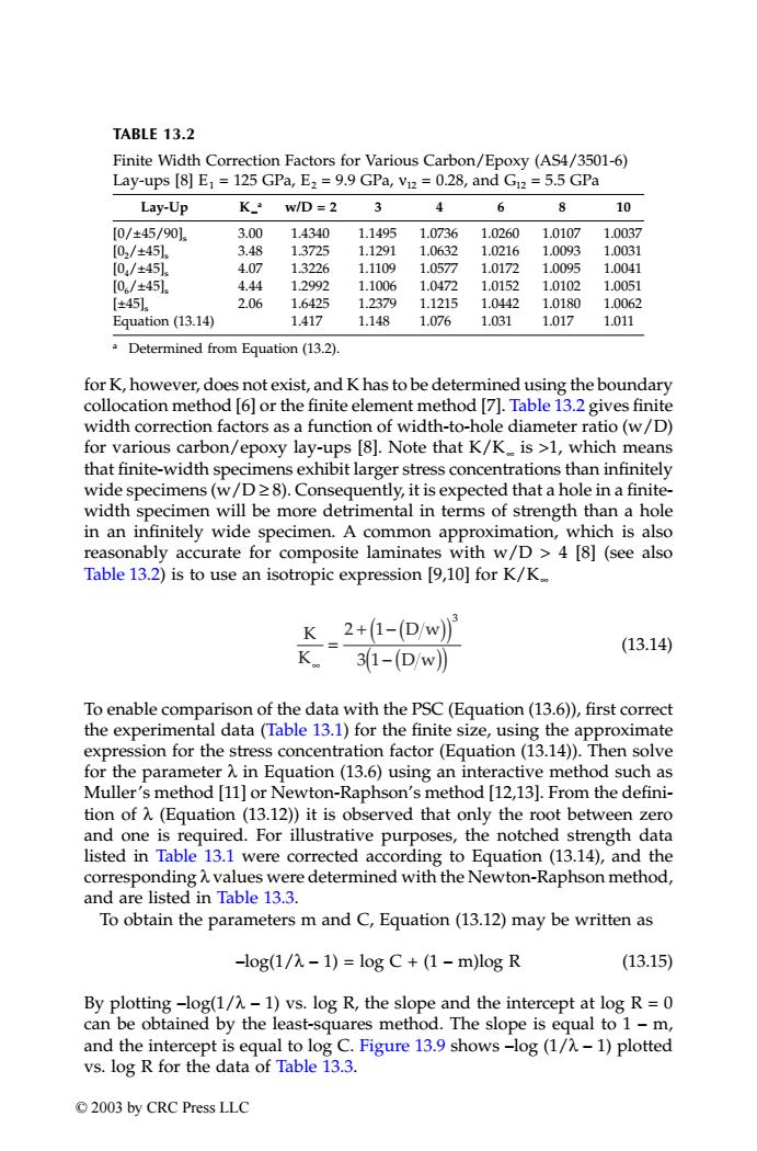
TABLE 13.2 Finite Width Correction Factors for Various Carbon/Epoxy(AS4/3501-6) Lay-ups [8]E1=125 GPa,E2 =9.9 GPa,Vi2=0.28,and Gu2 =5.5 GPa Lay-Up K w/D=2 6 8 10 [0/±45/901. 3.00 1.4340 1.1495 1.0736 1.0260 1.0107 1.0037 [02/±451. 3.48 1.3725 1.1291 1.0632 1.0216 1.0093 1.0031 [0/±45l. 4.07 1.3226 1.1109 1.0577 1.0172 1.0095 1.0041 [0./±451. 4.44 1.2992 1.1006 1.0472 1.0152 1.0102 1.0051 [±451l 2.06 1.6425 1.2379 1.1215 1.0442 1.0180 1.0062 Equation (13.14) 1.417 1.148 1.076 1.031 1.017 1.011 Determined from Equation(13.2). for K,however,does not exist,and K has to be determined using the boundary collocation method [6]or the finite element method [7].Table 13.2 gives finite width correction factors as a function of width-to-hole diameter ratio(w/D) for various carbon/epoxy lay-ups [8].Note that K/K is >1,which means that finite-width specimens exhibit larger stress concentrations than infinitely wide specimens(w/D28).Consequently,it is expected that a hole in a finite- width specimen will be more detrimental in terms of strength than a hole in an infinitely wide specimen.A common approximation,which is also reasonably accurate for composite laminates with w/D>4 [8](see also Table 13.2)is to use an isotropic expression [9,10]for K/K. K_2+1-(D/w) K31-(D/w)） (13.14) To enable comparison of the data with the PSC(Equation(13.6)),first correct the experimental data(Table 13.1)for the finite size,using the approximate expression for the stress concentration factor(Equation(13.14)).Then solve for the parameter A in Equation(13.6)using an interactive method such as Muller's method [11]or Newton-Raphson's method [12,13].From the defini- tion of A(Equation (13.12))it is observed that only the root between zero and one is required.For illustrative purposes,the notched strength data listed in Table 13.1 were corrected according to Equation(13.14),and the corresponding A values were determined with the Newton-Raphson method, and are listed in Table 13.3. To obtain the parameters m and C,Equation(13.12)may be written as -log(1/-1)=log C+(1-m)log R (13.15) By plotting-log(1/-1)vs.log R,the slope and the intercept at log R=0 can be obtained by the least-squares method.The slope is equal to 1-m, and the intercept is equal to log C.Figure 13.9 shows -log (1/A-1)plotted vs.log R for the data of Table 13.3. ©2003 by CRC Press LLCfor K, however, does not exist, and K has to be determined using the boundary collocation method [6] or the finite element method [7]. Table 13.2 gives finite width correction factors as a function of width-to-hole diameter ratio (w/D) for various carbon/epoxy lay-ups [8]. Note that K/K∞ is >1, which means that finite-width specimens exhibit larger stress concentrations than infinitely wide specimens (w/D ≥ 8). Consequently, it is expected that a hole in a finite￾width specimen will be more detrimental in terms of strength than a hole in an infinitely wide specimen. A common approximation, which is also reasonably accurate for composite laminates with w/D > 4 [8] (see also Table 13.2) is to use an isotropic expression [9,10] for K/K∞ (13.14) To enable comparison of the data with the PSC (Equation (13.6)), first correct the experimental data (Table 13.1) for the finite size, using the approximate expression for the stress concentration factor (Equation (13.14)). Then solve for the parameter λ in Equation (13.6) using an interactive method such as Muller’s method [11] or Newton-Raphson’s method [12,13]. From the defini￾tion of λ (Equation (13.12)) it is observed that only the root between zero and one is required. For illustrative purposes, the notched strength data listed in Table 13.1 were corrected according to Equation (13.14), and the corresponding λ values were determined with the Newton-Raphson method, and are listed in Table 13.3. To obtain the parameters m and C, Equation (13.12) may be written as –log(1/λ – 1) = log C + (1 – m)log R (13.15) By plotting –log(1/λ – 1) vs. log R, the slope and the intercept at log R = 0 can be obtained by the least-squares method. The slope is equal to 1 – m, and the intercept is equal to log C. Figure 13.9 shows –log (1/λ – 1) plotted vs. log R for the data of Table 13.3. TABLE 13.2 Finite Width Correction Factors for Various Carbon/Epoxy (AS4/3501-6) Lay-ups [8] E1 = 125 GPa, E2 = 9.9 GPa, ν12 = 0.28, and G12 = 5.5 GPa Lay-Up K∞ a w/D = 2 3 4 6 8 10 [0/±45/90]s [02/±45]s [04/±45]s [06/±45]s [±45]s Equation (13.14) 3.00 3.48 4.07 4.44 2.06 1.4340 1.3725 1.3226 1.2992 1.6425 1.417 1.1495 1.1291 1.1109 1.1006 1.2379 1.148 1.0736 1.0632 1.0577 1.0472 1.1215 1.076 1.0260 1.0216 1.0172 1.0152 1.0442 1.031 1.0107 1.0093 1.0095 1.0102 1.0180 1.017 1.0037 1.0031 1.0041 1.0051 1.0062 1.011 a Determined from Equation (13.2). K K 2 Dw ∞ D w = + − ( ) ( ) ( ) − ( ) 1 3 1 3 TX001_ch13_Frame Page 177 Saturday, September 21, 2002 5:07 AM © 2003 by CRC Press LLC