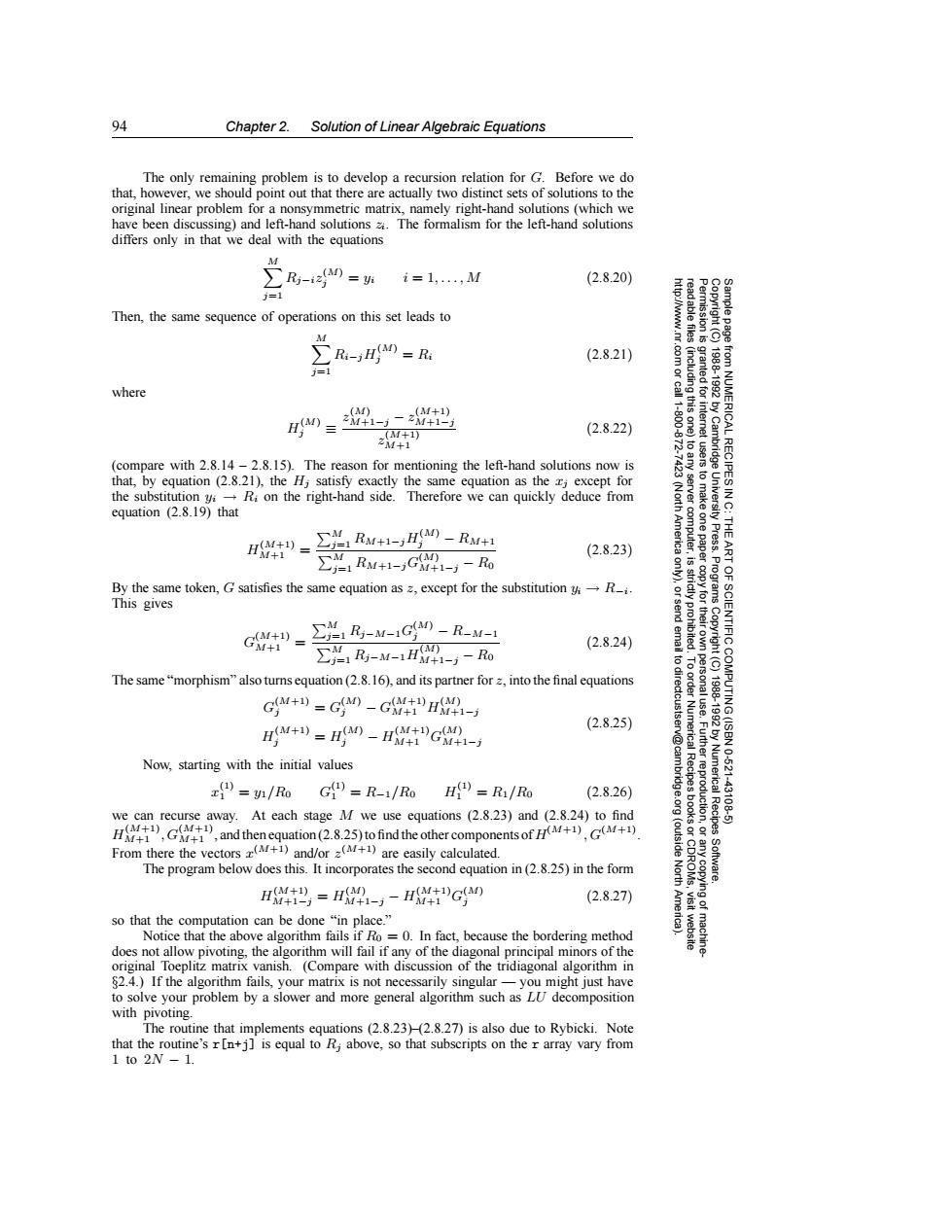
94 Chapter 2.Solution of Linear Algebraic Equations The only remaining problem is to develop a recursion relation for G.Before we do that,however,we should point out that there are actually two distinct sets of solutions to the original linear problem for a nonsymmetric matrix,namely right-hand solutions(which we have been discussing)and left-hand solutions.The formalism for the left-hand solutions differs only in that we deal with the equations ∑R-0=h i=1,,M (2.8.20) j= Then,the same sequence of operations on this set leads to ∑R-H=R (2.8.21) j= where 4--4出 (M) 三 (2.8.22) (compare with 2.8.14-2.8.15).The reason for mentioning the left-hand solutions now is that,by equation (2.8.21),the Hj satisfy exactly the same equation as the j except for RECIPES the substitution yaRi on the right-hand side. Therefore we can quickly deduce from equation (2.8.19)that 4= ∑01RM+1-H-RM+1 M (2.8.23) Press. 1RaM+1-G+1-)-Bo 9 By the same token,G satisfies the same equation as z,except for the substitution yR. 9 This gives G4= ∑R-M-1G0-R-M- (2.8.24) IENTIFIC M ∑g-M-1H4--Ro The same"morphism"also turns equation(2.8.16),and its partner for z,into the final equations GM)=)-G (M) 4+=0-H4c- (2.8.25) (ISBN Now,starting with the initial values )=y/Ro G)=R-1/Ro H)=Ri/Ro Numerical (2.8.26) ucti -43126 we can recurse away.At each stage M we use equations (2.8.23)and (2.8.24)to find ,and then equation(2.8.25)to find the other components of ) Recipes From there the vectors(M+)and/or (+1)are easily calculated. The program below does this.It incorporates the second equation in(2.8.25)in the form H巴，=4-，-H4G (2.8.27) so that the computation can be done“in place.” 香 Notice that the above algorithm fails if Ro =0.In fact,because the bordering method does not allow pivoting,the algorithm will fail if any of the diagonal principal minors of the original Toeplitz matrix vanish.(Compare with discussion of the tridiagonal algorithm in 82.4.)If the algorithm fails,your matrix is not necessarily singular-you might just have to solve your problem by a slower and more general algorithm such as LU decomposition with pivoting. The routine that implements equations(2.8.23)(2.8.27)is also due to Rybicki.Note that the routine's r[n+j]is equal to Rj above,so that subscripts on the r array vary from 1to2N-1.94 Chapter 2. Solution of Linear Algebraic Equations Permission is granted for internet users to make one paper copy for their own personal use. Further reproduction, or any copyin Copyright (C) 1988-1992 by Cambridge University Press. Programs Copyright (C) 1988-1992 by Numerical Recipes Software. Sample page from NUMERICAL RECIPES IN C: THE ART OF SCIENTIFIC COMPUTING (ISBN 0-521-43108-5) g of machine￾readable files (including this one) to any server computer, is strictly prohibited. To order Numerical Recipes books or CDROMs, visit website http://www.nr.com or call 1-800-872-7423 (North America only), or send email to directcustserv@cambridge.org (outside North America). The only remaining problem is to develop a recursion relation for G. Before we do that, however, we should point out that there are actually two distinct sets of solutions to the original linear problem for a nonsymmetric matrix, namely right-hand solutions (which we have been discussing) and left-hand solutions zi. The formalism for the left-hand solutions differs only in that we deal with the equations M j=1 Rj−iz(M) j = yi i = 1,...,M (2.8.20) Then, the same sequence of operations on this set leads to M j=1 Ri−jH(M) j = Ri (2.8.21) where H(M) j ≡ z (M) M+1−j − z(M+1) M+1−j z(M+1) M+1 (2.8.22) (compare with 2.8.14 – 2.8.15). The reason for mentioning the left-hand solutions now is that, by equation (2.8.21), the Hj satisfy exactly the same equation as the xj except for the substitution yi → Ri on the right-hand side. Therefore we can quickly deduce from equation (2.8.19) that H(M+1) M+1 = M j=1 RM+1−jH(M) j − RM+1 M j=1 RM+1−jG(M) M+1−j − R0 (2.8.23) By the same token, G satisfies the same equation as z, except for the substitution yi → R−i. This gives G(M+1) M+1 = M j=1 Rj−M−1G(M) j − R−M−1 M j=1 Rj−M−1H(M) M+1−j − R0 (2.8.24) The same “morphism” also turns equation (2.8.16), and its partner for z, into the final equations G(M+1) j = G(M) j − G(M+1) M+1 H(M) M+1−j H(M+1) j = H(M) j − H(M+1) M+1 G(M) M+1−j (2.8.25) Now, starting with the initial values x(1) 1 = y1/R0 G(1) 1 = R−1/R0 H(1) 1 = R1/R0 (2.8.26) we can recurse away. At each stage M we use equations (2.8.23) and (2.8.24) to find H(M+1) M+1 , G(M+1) M+1 , and then equation (2.8.25) to find the other components of H(M+1) , G(M+1). From there the vectors x(M+1) and/or z(M+1) are easily calculated. The program below does this. It incorporates the second equation in (2.8.25) in the form H(M+1) M+1−j = H(M) M+1−j − H(M+1) M+1 G(M) j (2.8.27) so that the computation can be done “in place.” Notice that the above algorithm fails if R0 = 0. In fact, because the bordering method does not allow pivoting, the algorithm will fail if any of the diagonal principal minors of the original Toeplitz matrix vanish. (Compare with discussion of the tridiagonal algorithm in §2.4.) If the algorithm fails, your matrix is not necessarily singular — you might just have to solve your problem by a slower and more general algorithm such as LU decomposition with pivoting. The routine that implements equations (2.8.23)–(2.8.27) is also due to Rybicki. Note that the routine’s r[n+j] is equal to Rj above, so that subscripts on the r array vary from 1 to 2N − 1