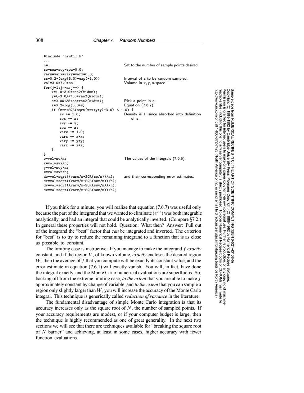
308 Chapter 7. Random Numbers #include "nrutil.h" ns... Set to the number of sample points desired. sw=swx=swy=swz=0.0; varw=varx=vary=varz-0.0; ss=0.2*(exp(5.0)-exp(-5.0)) Interval of s to be random sampled. v01=3.0*7.0*gs Volume in x,y,s-space. for(j=1;j<=m;j++) x=1.0+3.0*ran2(&1dum); y=(-3.0)+7.0*ran2(&idum); s=0.00135+ss*ran2(&idum); Pick a point in s. z=0.2*10g(5.0*s); Equation (7.6.7). 1f(z*z+SqR(sqrt(x*x+y*y)-3.0)<1.0)[ sw+=1.0; Density is 1,since absorbed into definition SWX +x; of s. swy +yi 鱼 18881892 SWZ +Z; varw +1.0; 1-800 varx +x*x; vary +=y*yi varz +z*Z; from NUMERICAL RECIPES I w=vol*sw/n; The values of the integrals (7.6.5). x=Vol米swx/n; y=vol*swy/n; z=vol*swz/n; Americ computer, Press. dw=vol*sqrt((varw/n-SQR(sw/n))/n); and their corresponding error estimates. ART dx=vol*sqrt((varx/n-SQR(swx/n))/n); dy=vol*sqrt((vary/n-SQR(swy/n))/n); dz=vol*sqrt((varz/n-SQR(swz/n))/n); 9 Programs SCIENTIFIC If you think for a minute,you will realize that equation(7.6.7)was useful only because the part of the integrand that we wanted to eliminate(e5=)was both integrable analytically,and had an integral that could be analytically inverted.(Compare 87.2.) In general these properties will not hold.Question:What then?Answer:Pull out of the integrand the "best"factor that can be integrated and inverted.The criterion for "best"is to try to reduce the remaining integrand to a function that is as close as possible to constant. 10-621 The limiting case is instructive:If you manage to make the integrand f exactly Numerical constant,and if the region V,of known volume,exactly encloses the desired region W,then the average of f that you compute will be exactly its constant value,and the Recipes 43106 error estimate in equation(7.6.1)will exactly vanish.You will,in fact,have done the integral exactly,and the Monte Carlo numerical evaluations are superfluous.So, (outside backing off from the extreme limiting case,to the extent that you are able to make f North Software. approximately constant by change of variable,and to the extent that you can sample a region only slightly larger than W,you will increase the accuracy of the Monte Carlo integral.This technique is generically called reduction of variance in the literature. The fundamental disadvantage of simple Monte Carlo integration is that its accuracy increases only as the square root of N.the number of sampled points.If your accuracy requirements are modest,or if your computer budget is large,then the technique is highly recommended as one of great generality.In the next two sections we will see that there are techniques available for "breaking the square root of N barrier"and achieving,at least in some cases,higher accuracy with fewer function evaluations.308 Chapter 7. Random Numbers Permission is granted for internet users to make one paper copy for their own personal use. Further reproduction, or any copyin Copyright (C) 1988-1992 by Cambridge University Press. Programs Copyright (C) 1988-1992 by Numerical Recipes Software. Sample page from NUMERICAL RECIPES IN C: THE ART OF SCIENTIFIC COMPUTING (ISBN 0-521-43108-5) g of machine￾readable files (including this one) to any server computer, is strictly prohibited. To order Numerical Recipes books or CDROMs, visit website http://www.nr.com or call 1-800-872-7423 (North America only), or send email to directcustserv@cambridge.org (outside North America). #include "nrutil.h" ... n=... Set to the number of sample points desired. sw=swx=swy=swz=0.0; varw=varx=vary=varz=0.0; ss=0.2*(exp(5.0)-exp(-5.0)) Interval of s to be random sampled. vol=3.0*7.0*ss Volume in x,y,s-space. for(j=1;j<=n;j++) { x=1.0+3.0*ran2(&idum); y=(-3.0)+7.0*ran2(&idum); s=0.00135+ss*ran2(&idum); Pick a point in s. z=0.2*log(5.0*s); Equation (7.6.7). if (z*z+SQR(sqrt(x*x+y*y)-3.0) < 1.0) { sw += 1.0; Density is 1, since absorbed into definition swx += x; of s. swy += y; swz += z; varw += 1.0; varx += x*x; vary += y*y; varz += z*z; } } w=vol*sw/n; The values of the integrals (7.6.5), x=vol*swx/n; y=vol*swy/n; z=vol*swz/n; dw=vol*sqrt((varw/n-SQR(sw/n))/n); and their corresponding error estimates. dx=vol*sqrt((varx/n-SQR(swx/n))/n); dy=vol*sqrt((vary/n-SQR(swy/n))/n); dz=vol*sqrt((varz/n-SQR(swz/n))/n); If you think for a minute, you will realize that equation (7.6.7) was useful only because the part of the integrand that we wanted to eliminate (e 5z) was both integrable analytically, and had an integral that could be analytically inverted. (Compare §7.2.) In general these properties will not hold. Question: What then? Answer: Pull out of the integrand the “best” factor that can be integrated and inverted. The criterion for “best” is to try to reduce the remaining integrand to a function that is as close as possible to constant. The limiting case is instructive: If you manage to make the integrand f exactly constant, and if the region V , of known volume, exactly encloses the desired region W, then the average of f that you compute will be exactly its constant value, and the error estimate in equation (7.6.1) will exactly vanish. You will, in fact, have done the integral exactly, and the Monte Carlo numerical evaluations are superfluous. So, backing off from the extreme limiting case, to the extent that you are able to make f approximately constant by change of variable, and to the extent that you can sample a region only slightly larger than W, you will increase the accuracy of the Monte Carlo integral. This technique is generically called reduction of variance in the literature. The fundamental disadvantage of simple Monte Carlo integration is that its accuracy increases only as the square root of N, the number of sampled points. If your accuracy requirements are modest, or if your computer budget is large, then the technique is highly recommended as one of great generality. In the next two sections we will see that there are techniques available for “breaking the square root of N barrier” and achieving, at least in some cases, higher accuracy with fewer function evaluations