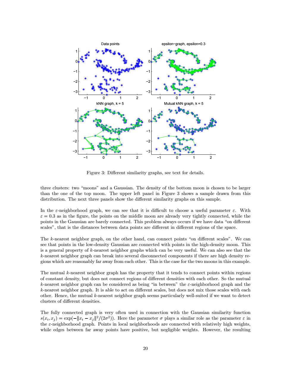
Data points epsilon-graph,epsilon=0.3 kNN grapr Mutual kNN graph,k =5 Figure 3:Different similarity graphs,see text for details. three clusters:two "moons"and a Gaussian.The density of the bottom moon is chosen to be larger than the one of the top moon.The upper left panel in Figure 3 shows a sample drawn from this distribution.The next three panels show the different similarity graphs on this sample. In the e-neighborhood graph,we can see that it is difficult to choose a useful parameter s.With s=0.3 as in the figure,the points on the middle moon are already very tightly connected,while the points in the Gaussian are barely connected.This problem always occurs if we have data "on different scales",that is the distances between data points are different in different regions of the space. The k-nearest neighbor graph,on the other hand,can connect points "on different scales".We can see that points in the low-density Gaussian are connected with points in the high-density moon.This is a general property of k-nearest neighbor graphs which can be very useful.We can also see that the k-nearest neighbor graph can break into several disconnected components if there are high density re- gions which are reasonably far away from each other.This is the case for the two moons in this example. The mutual k-nearest neighbor graph has the property that it tends to connect points within regions of constant density,but does not connect regions of different densities with each other.So the mutual k-nearest neighbor graph can be considered as being "in between"the s-neighborhood graph and the k-nearest neighbor graph.It is able to act on different scales,but does not mix those scales with each other.Hence,the mutual k-nearest neighbor graph seems particularly well-suited if we want to detect clusters of different densities. The fully connected graph is very often used in connection with the Gaussian similarity function s(ri,j)=exp(-llti-jll2/(202)).Here the parameter o plays a similar role as the parameter in the s-neighborhood graph.Points in local neighborhoods are connected with relatively high weights, while edges between far away points have positive,but negligible weights.However,the resulting 20−1 0 1 2 −3 −2 −1 0 1 Data points −1 0 1 2 −3 −2 −1 0 1 epsilon−graph, epsilon=0.3 −1 0 1 2 −3 −2 −1 0 1 kNN graph, k = 5 −1 0 1 2 −3 −2 −1 0 1 Mutual kNN graph, k = 5 Figure 3: Different similarity graphs, see text for details. three clusters: two “moons” and a Gaussian. The density of the bottom moon is chosen to be larger than the one of the top moon. The upper left panel in Figure 3 shows a sample drawn from this distribution. The next three panels show the different similarity graphs on this sample. In the ε-neighborhood graph, we can see that it is difficult to choose a useful parameter ε. With ε = 0.3 as in the figure, the points on the middle moon are already very tightly connected, while the points in the Gaussian are barely connected. This problem always occurs if we have data “on different scales”, that is the distances between data points are different in different regions of the space. The k-nearest neighbor graph, on the other hand, can connect points “on different scales”. We can see that points in the low-density Gaussian are connected with points in the high-density moon. This is a general property of k-nearest neighbor graphs which can be very useful. We can also see that the k-nearest neighbor graph can break into several disconnected components if there are high density re￾gions which are reasonably far away from each other. This is the case for the two moons in this example. The mutual k-nearest neighbor graph has the property that it tends to connect points within regions of constant density, but does not connect regions of different densities with each other. So the mutual k-nearest neighbor graph can be considered as being “in between” the ε-neighborhood graph and the k-nearest neighbor graph. It is able to act on different scales, but does not mix those scales with each other. Hence, the mutual k-nearest neighbor graph seems particularly well-suited if we want to detect clusters of different densities. The fully connected graph is very often used in connection with the Gaussian similarity function s(xi , xj ) = exp(−kxi − xjk 2/(2σ 2 )). Here the parameter σ plays a similar role as the parameter ε in the ε-neighborhood graph. Points in local neighborhoods are connected with relatively high weights, while edges between far away points have positive, but negligible weights. However, the resulting 20