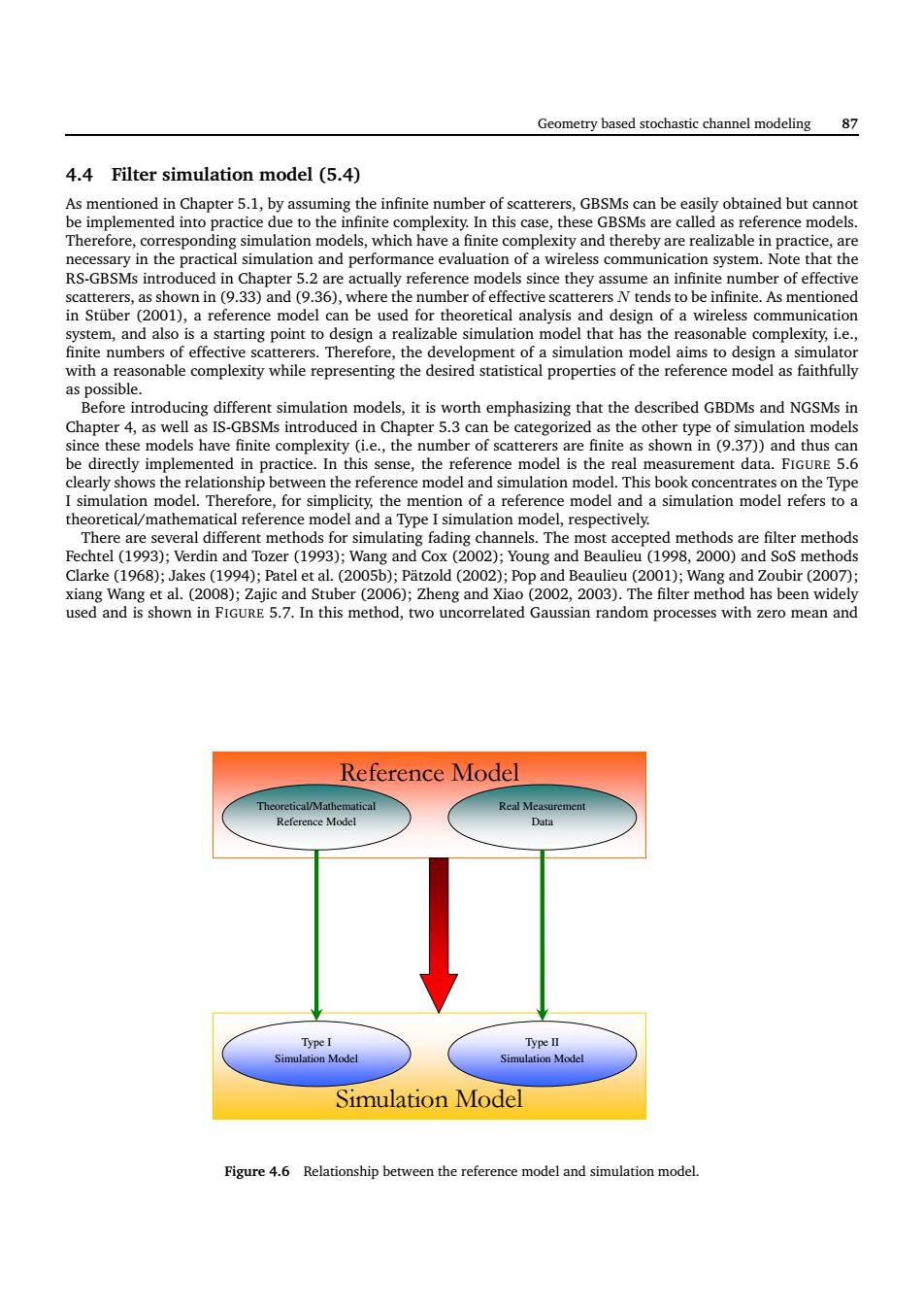
Geometry based stochastic channel modeling 87 4.4 Filter simulation model(5.4) gBSMs can be ea sily obtained but canno 35 reference models. which have a finiteco plexity and thereby are realizable in pra me an infinite number of effective scatte end to b ystem,and also is a starting point to design a realizable simulation model that has the reasonable complexit properties d as dels,it is w orth emphasizing that the described GBDMs and NGSMs in simulation model The refore,for simplicity,the mention of a referer e model and a simulation model refers to Clarke(1968); akes(Parelet al ()()Pop and Be (1)Wang and our( used and is shown in.7.In this method,two uncorrelated Gaussian randon cesses with zero mean and Reference Model Simulation Model Figure 4.6 Relationship between the reference model and simulation modelGeometry based stochastic channel modeling 87 4.4 Filter simulation model (5.4) As mentioned in Chapter 5.1, by assuming the infinite number of scatterers, GBSMs can be easily obtained but cannot be implemented into practice due to the infinite complexity. In this case, these GBSMs are called as reference models. Therefore, corresponding simulation models, which have a finite complexity and thereby are realizable in practice, are necessary in the practical simulation and performance evaluation of a wireless communication system. Note that the RS-GBSMs introduced in Chapter 5.2 are actually reference models since they assume an infinite number of effective scatterers, as shown in (9.33) and (9.36), where the number of effective scatterers N tends to be infinite. As mentioned in Stüber (2001), a reference model can be used for theoretical analysis and design of a wireless communication system, and also is a starting point to design a realizable simulation model that has the reasonable complexity, i.e., finite numbers of effective scatterers. Therefore, the development of a simulation model aims to design a simulator with a reasonable complexity while representing the desired statistical properties of the reference model as faithfully as possible. Before introducing different simulation models, it is worth emphasizing that the described GBDMs and NGSMs in Chapter 4, as well as IS-GBSMs introduced in Chapter 5.3 can be categorized as the other type of simulation models since these models have finite complexity (i.e., the number of scatterers are finite as shown in (9.37)) and thus can be directly implemented in practice. In this sense, the reference model is the real measurement data. FIGURE 5.6 clearly shows the relationship between the reference model and simulation model. This book concentrates on the Type I simulation model. Therefore, for simplicity, the mention of a reference model and a simulation model refers to a theoretical/mathematical reference model and a Type I simulation model, respectively. There are several different methods for simulating fading channels. The most accepted methods are filter methods Fechtel (1993); Verdin and Tozer (1993); Wang and Cox (2002); Young and Beaulieu (1998, 2000) and SoS methods Clarke (1968); Jakes (1994); Patel et al. (2005b); Pätzold (2002); Pop and Beaulieu (2001); Wang and Zoubir (2007); xiang Wang et al. (2008); Zajic and Stuber (2006); Zheng and Xiao (2002, 2003). The filter method has been widely used and is shown in FIGURE 5.7. In this method, two uncorrelated Gaussian random processes with zero mean and Reference Model Simulation Model Real Measurement Data Type I Simulation Model Type II Simulation Model Theoretical/Mathematical Reference Model Figure 4.6 Relationship between the reference model and simulation model