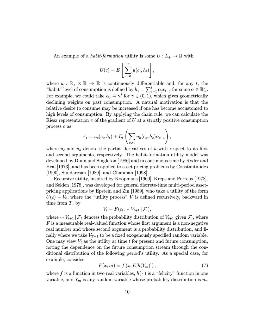
An example of a habit-formation utility is some U:L+-R with U(c) uc.h) where u:R+x R->R is continuously differentiable and,for any t,the habit"level of consumption is defined by for some For example,we could take aj=y for y(0,1),which gives geometrically declining weights on past consumption.A natural motivation is that the relative desire to consume may be increased if one has become accustomed to high levels of consumption.By applying the chain rule,we can calculate the Riesz representation m of the gradient of U at a strictly positive consumption process c as Tt ue(ct;ht)+E un(Cs;hs)as-t s>t where uc and un denote the partial derivatives of u with respect to its first and second arguments,respectively.The habit-formation utility model was developed by Dunn and Singleton [1986 and in continuous time by Ryder and Heal [1973],and has been applied to asset pricing problems by Constantinides [1990],Sundaresan [1989],and Chapman [1998]. Recursive utility,inspired by Koopmans [1960],Kreps and Porteus [1978], and Selden [1978,was developed for general discrete-time multi-period asset- pricing applications by Epstein and Zin [1989],who take a utility of the form U(c)=Vo,where the "utility process"V is defined recursively,backward in time from T,by Vi=F(c~V+F), whereV+F denotes the probability distribution of V+i given F,where F is a measurable real-valued function whose first argument is a non-negative real number and whose second argument is a probability distribution,and fi- nally where we take Vr-to be a fixed exogenously specified random variable. One may view Vi as the utility at time t for present and future consumption, noting the dependence on the future consumption stream through the con- ditional distribution of the following period's utility.As a special case,for example,consider F(x,m)=f(,E[h(Ym)), (7) where f is a function in two real variables,h(.)is a "felicity"function in one variable,and Ym is any random variable whose probability distribution is m. 10An example of a habit-formation utility is some U : L+ → R with U(c) = E " X T t=0 u(ct, ht) # , where u : R+ × R → R is continuously differentiable and, for any t, the “habit” level of consumption is defined by ht = Pt j=1 αj ct−j for some α ∈ RT +. For example, we could take αj = γj for γ ∈ (0, 1), which gives geometrically declining weights on past consumption. A natural motivation is that the relative desire to consume may be increased if one has become accustomed to high levels of consumption. By applying the chain rule, we can calculate the Riesz representation π of the gradient of U at a strictly positive consumption process c as πt = uc(ct, ht) + Et X s>t uh(cs, hs)αs−t ! , where uc and uh denote the partial derivatives of u with respect to its first and second arguments, respectively. The habit-formation utility model was developed by Dunn and Singleton [1986] and in continuous time by Ryder and Heal [1973], and has been applied to asset pricing problems by Constantinides [1990], Sundaresan [1989], and Chapman [1998]. Recursive utility, inspired by Koopmans [1960], Kreps and Porteus [1978], and Selden [1978], was developed for general discrete-time multi-period asset￾pricing applications by Epstein and Zin [1989], who take a utility of the form U(c) = V0, where the “utility process” V is defined recursively, backward in time from T, by Vt = F(ct, ∼ Vt+1 | Ft), where ∼ Vt+1 | Ft denotes the probability distribution of Vt+1 given Ft, where F is a measurable real-valued function whose first argument is a non-negative real number and whose second argument is a probability distribution, and fi- nally where we take VT +1 to be a fixed exogenously specified random variable. One may view Vt as the utility at time t for present and future consumption, noting the dependence on the future consumption stream through the con￾ditional distribution of the following period’s utility. As a special case, for example, consider F(x, m) = f (x, E[h(Ym)]), (7) where f is a function in two real variables, h(·) is a “felicity” function in one variable, and Ym is any random variable whose probability distribution is m. 10