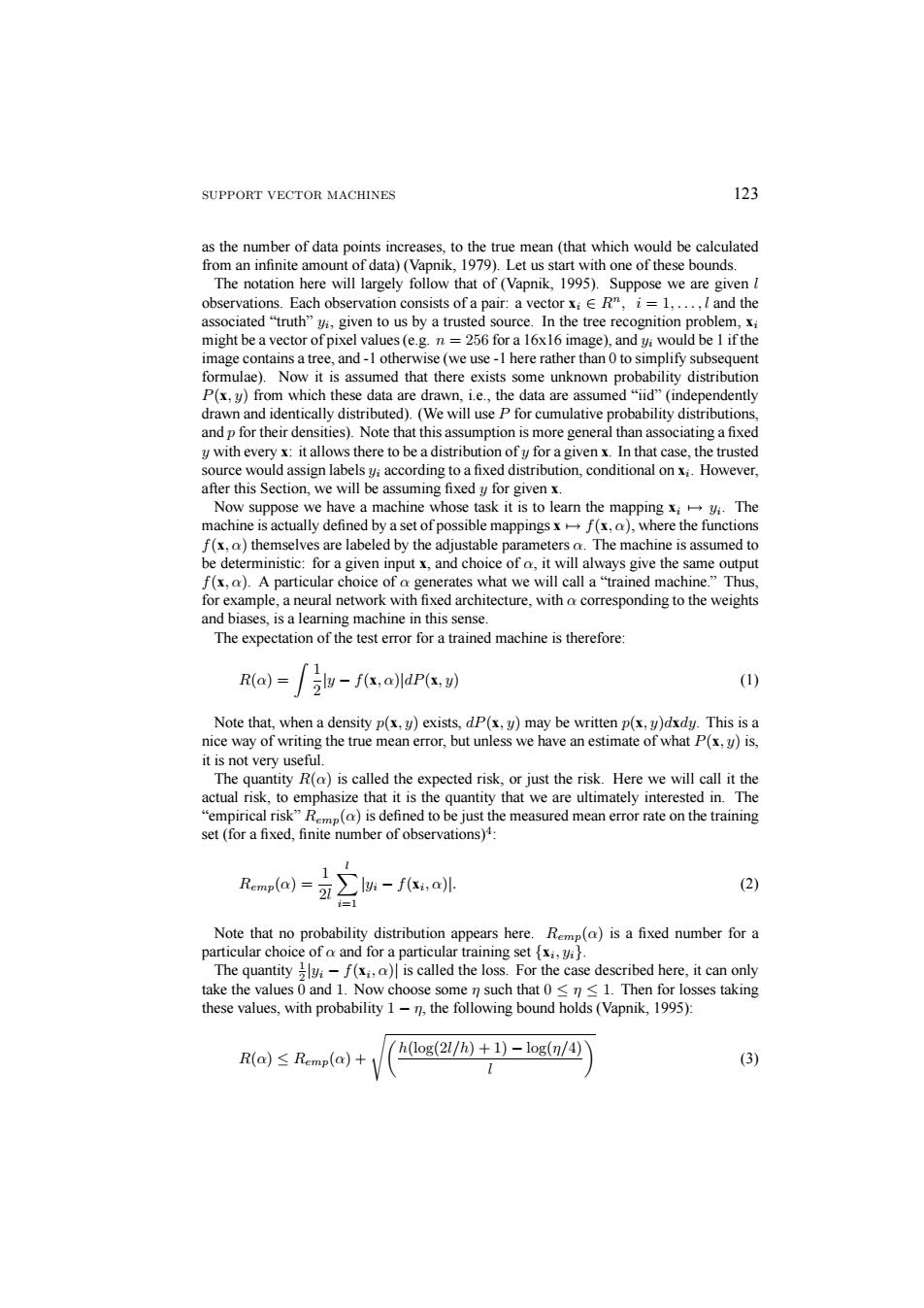
SUPPORT VECTOR MACHINES 123 as the number of data points increases,to the true mean (that which would be calculated from an infinite amount of data)(Vapnik,1979).Let us start with one of these bounds The notation here will largely follow that of (Vapnik,1995).Suppose we are given l observations.Each observation consists of a pair:a vector xiE R",i=1....,l and the associated "truth"yi,given to us by a trusted source.In the tree recognition problem,xi might be a vector of pixel values(e.g.n=256 for a 16x16 image),and yi would be 1 if the image contains a tree,and-1 otherwise(we use-1 here rather than 0 to simplify subsequent formulae).Now it is assumed that there exists some unknown probability distribution P(x,y)from which these data are drawn,ie.,the data are assumed"iid"(independently drawn and identically distributed).(We will use P for cumulative probability distributions and p for their densities).Note that this assumption is more general than associating a fixed y with every x:it allows there to be a distribution ofy for a given x.In that case,the trusted source would assign labelsyi according to a fixed distribution,conditional on x.However, after this Section,we will be assuming fixed y for given x. Now suppose we have a machine whose task it is to learn the mapping xiy The machine is actually defined by a set of possible mappings xf(x,)where the functions f(x,a)themselves are labeled by the adjustable parameters a.The machine is assumed to be deterministic:for a given input x,and choice of o,it will always give the same output f(x,a).A particular choice of a generates what we will call a"trained machine."Thus. for example,a neural network with fixed architecture.with a corresponding to the weights and biases,is a learning machine in this sense The expectation of the test error for a trained machine is therefore: R(a)=l-f(x,a)ldP(x.) (1) Note that,when a density p(x,y)exists,dP(x,y)may be written p(x,y)dxdy.This is a nice way of writing the true mean error,but unless we have an estimate of what P(x,y)is, it is not very useful The quantity R(a)is called the expected risk,or just the risk.Here we will call it the actual risk,to emphasize that it is the quantity that we are ultimately interested in.The "empirical risk"R()is defined to be just the measured mean error rate on the training set(for a fixed,finite number of observations)4: Remp(a)= ∑l-fk,al (2) =1 Note that no probability distribution appears here.Remp(a)is a fixed number for a particular choice of a and for a particular training set {x,y. The quantity-f(xi,a)is called the loss.For the case described here,it can only take the values 0 and 1.Now choose some n such that 0<n<1.Then for losses taking these values,with probability 1-n,the following bound holds(Vapnik,1995): R(a)≤Remp(a)+ h(log(21/h)+1)-log(n/4) (3)SUPPORT VECTOR MACHINES 123 as the number of data points increases, to the true mean (that which would be calculated from an infinite amount of data) (Vapnik, 1979). Let us start with one of these bounds. The notation here will largely follow that of (Vapnik, 1995). Suppose we are given l observations. Each observation consists of a pair: a vector xi ∈ Rn, i = 1,...,l and the associated “truth” yi, given to us by a trusted source. In the tree recognition problem, xi might be a vector of pixel values (e.g. n = 256 for a 16x16 image), and yi would be 1 if the image contains a tree, and -1 otherwise (we use -1 here rather than 0 to simplify subsequent formulae). Now it is assumed that there exists some unknown probability distribution P(x, y) from which these data are drawn, i.e., the data are assumed “iid” (independently drawn and identically distributed). (We will use P for cumulative probability distributions, and p for their densities). Note that this assumption is more general than associating a fixed y with every x: it allows there to be a distribution of y for a given x. In that case, the trusted source would assign labels yi according to a fixed distribution, conditional on xi. However, after this Section, we will be assuming fixed y for given x. Now suppose we have a machine whose task it is to learn the mapping xi 7→ yi. The machine is actually defined by a set of possible mappings x 7→ f(x, α), where the functions f(x, α) themselves are labeled by the adjustable parameters α. The machine is assumed to be deterministic: for a given input x, and choice of α, it will always give the same output f(x, α). A particular choice of α generates what we will call a “trained machine.” Thus, for example, a neural network with fixed architecture, with α corresponding to the weights and biases, is a learning machine in this sense. The expectation of the test error for a trained machine is therefore: R(α) = Z 1 2 |y − f(x, α)|dP(x, y) (1) Note that, when a density p(x, y) exists, dP(x, y) may be written p(x, y)dxdy. This is a nice way of writing the true mean error, but unless we have an estimate of what P(x, y) is, it is not very useful. The quantity R(α) is called the expected risk, or just the risk. Here we will call it the actual risk, to emphasize that it is the quantity that we are ultimately interested in. The “empirical risk” Remp(α) is defined to be just the measured mean error rate on the training set (for a fixed, finite number of observations)4: Remp(α) = 1 2l X l i=1 |yi − f(xi, α)|. (2) Note that no probability distribution appears here. Remp(α) is a fixed number for a particular choice of α and for a particular training set {xi, yi}. The quantity 1 2 |yi − f(xi, α)| is called the loss. For the case described here, it can only take the values 0 and 1. Now choose some η such that 0 ≤ η ≤ 1. Then for losses taking these values, with probability 1 − η, the following bound holds (Vapnik, 1995): R(α) ≤ Remp(α) + sµh(log(2l/h) + 1) − log(η/4) l ¶ (3)