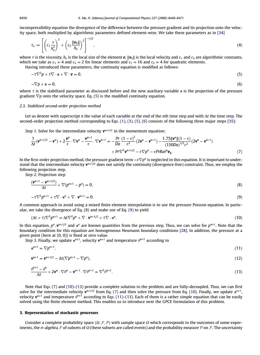
8450 X Ma,N.Zabaras foumal of Computational Physics 227(2008)8448-8471 incompressibility ation the div ce of the differ 1-12 (4 where is the viscosity,h is the local size of the elemente.is the local velocity and c and cz are algorithmic constants. -tV2p+tV,r+又.v=0. -Vp+π=0. (6) d the 2.3.Stabilized second-order projection method Step 1.Solve for the intermediate velocityin the momentum equation: +PrV2v+R-eVp"-cPrRaleg. Step 2.Projection step (8) -+tV.+V.=0. A2oeaChcmc2尚gacomDgsoeepmeeRaaaquieanunk (+t)2p+1=2+,v+n+t, (10) Step 3.Finally.we update,velocity y+and temperature according to 1=了p+1 (11) v1=viR -At(Vp1-Vp"). (12) +1- A +2.了0--1.了0m-1=2+1 (13) pled.Thus.we can firs 3.Representation of stochastic processes Consider a complete probability space(1.F.P)with sample space which corresponds to the outcomes of some exp iments.the a-algebraFof subsets of(these subsets are called events)and the probability measure PonF.The uncertaintyincompressibility equation the divergence of the difference between the pressure gradient and its projection onto the veloc￾ity space, both multiplied by algorithmic parameters defined element-wise. We take these parameters as in [34] se :¼ c1 m h2 e !2 þ c2 kvhk he 2 2 4 3 5 1=2 ; ð4Þ where m is the viscosity, he is the local size of the element e, kvhk is the local velocity and c1 and c2 are algorithmic constants, which we take as c1 ¼ 4 and c2 ¼ 2 for linear elements and c1 ¼ 16 and c2 ¼ 4 for quadratic elements. Having introduced these parameters, the continuity equation is modified as follows: sr2 p þ sr p þ r v ¼ 0; ð5Þ rp þ p ¼ 0; ð6Þ where s is the stabilized parameter as discussed before and the new auxiliary variable p is the projection of the pressure gradient rp onto the velocity space. Eq. (5) is the modified continuity equation. 2.3. Stabilized second-order projection method Let us denote with superscript n the value of each variable at the end of the nth time step and with Dt the time step. The second-order projection method corresponding to Eqs. (1), (3), (5), (6) consists of the following three major steps [35]: Step 1. Solve for the intermediate velocity vnþ1=2 in the momentum equation: 1 Dt ðvnþ1=2  vnÞ þ 2 vn rvn  vn1 rvn1 ¼  Pr Da ð1  Þ 2 2 ð2vn  vn1Þ  1:75kvnkð1  Þ ð150DaÞ 1=2 2 ð2vn  vn1Þ þ Prr2 vnþ1=2  rpn  PrRahn eg: ð7Þ In the first-order projection method, the pressure gradient term rpn is neglected in this equation. It is important to under￾stand that the intermediate velocity vnþ1=2 does not satisfy the continuity (divergence-free) constraint. Thus, we employ the following projection step. Step 2. Projection step ðvnþ1  vnþ1=2Þ Dt þ rðpnþ1  pnÞ ¼ 0; ð8Þ sr2 pnþ1 þ sr pn þ r vnþ1 ¼ 0: ð9Þ A common approach to avoid using a mixed finite element interpolation is to use the pressure Poisson equation. In partic￾ular, we take the divergence of Eq. (8) and make use of Eq. (9) to yield ðDt þ sÞr2 pnþ1 ¼ Dtr2 pn þ r vnþ1=2 þ sr pn: ð10Þ In this equation, pn; vnþ1=2 and pn are known quantities from the previous step. Thus, we can solve for pnþ1. Note that the boundary condition for this equation are homogeneous Neumann boundary conditions [28]. In addition, the pressure at a given point (here at (0, 0)) is fixed at zero value. Step 3. Finally, we update pnþ1, velocity vnþ1 and temperature hnþ1 according to pnþ1 ¼ rpnþ1; ð11Þ vnþ1 ¼ vnþ1=2  Dtðrpnþ1  rpnÞ; ð12Þ hnþ1  hn Dt þ 2vn rhn  vn1 rhn1 ¼ r2 hnþ1 : ð13Þ Note that Eqs. (7) and (10)–(13) provide a complete solution to the problem and are fully-decoupled. Thus, we can first solve for the intermediate velocity vnþ1=2 from Eq. (7) and then solve the pressure from Eq. (10). Finally, we update pnþ1, velocity vnþ1 and temperature hnþ1 according to Eqs. (11)–(13). Each of them is a rather simple equation that can be easily solved using the finite element method. This enables us to introduce next the GPCE formulation of this problem. 3. Representation of stochastic processes Consider a complete probability space ðX; F;PÞ with sample space X which corresponds to the outcomes of some exper￾iments, the r-algebra F of subsets of X (these subsets are called events) and the probability measure P on F. The uncertainty 8450 X. Ma, N. Zabaras / Journal of Computational Physics 227 (2008) 8448–8471