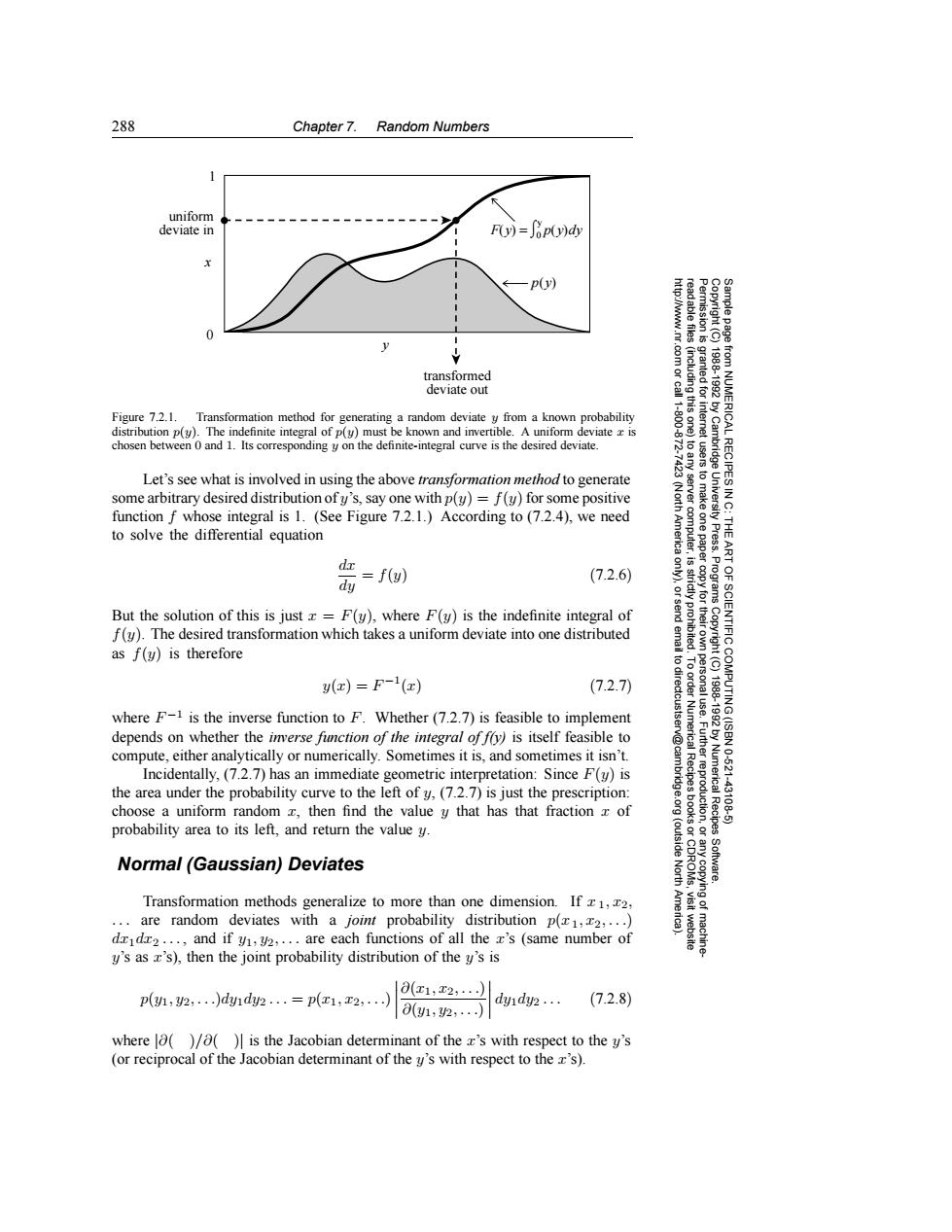
288 Chapter 7.Random Numbers uniform deviate in F(y)=Jop(y)dy -p(y) 0 transformed 83g deviate out Figure 7.2.1.Transformation method for generating a random deviate y from a known probability 1.800 distribution p(y).The indefinite integral of p(y)must be known and invertible.A uniform deviate x is chosen between 0 and 1.Its corresponding y on the definite-integral curve is the desired deviate. Let's see what is involved in using the above transformation method to generate some arbitrary desired distribution ofy's,say one with p(y)=f(y)for some positive function f whose integral is 1.(See Figure 7.2.1.)According to (7.2.4),we need to solve the differential equation Press. dx dy =f(u) (7.2.6) But the solution of this is just x =F(y),where F(y)is the indefinite integral of f(y).The desired transformation which takes a uniform deviate into one distributed IENTIFIC as f(y)is therefore 6 y(x)=F-1(x) (7.2.7) where F-1 is the inverse function to F.Whether(7.2.7)is feasible to implement 景影 depends on whether the inverse function of the integral of fry)is itself feasible to compute,either analytically or numerically.Sometimes it is,and sometimes it isn't. Incidentally,(7.2.7)has an immediate geometric interpretation:Since F(y)is Numerica 10.621 the area under the probability curve to the left of y,(7.2.7)is just the prescription: 431 choose a uniform random then find the value y that has that fraction x of E probability area to its left,and return the value y. (outside Recipes Normal(Gaussian)Deviates North Software. Transformation methods generalize to more than one dimension.If z1,z2, are random deviates with a joint probability distribution p(1,2,...) dzidr2...,and if y,y2,...are each functions of all the x's (same number of y's as z's),then the joint probability distribution of the y's is p(1,2,)d1d2.=p(x1,2,.) ∂(x1,x2,.】 dyidy2... (7.2.8) 01,2,） where o()/o(is the Jacobian determinant of the x's with respect to the y's (or reciprocal of the Jacobian determinant of the y's with respect to the z's).288 Chapter 7. Random Numbers Permission is granted for internet users to make one paper copy for their own personal use. Further reproduction, or any copyin Copyright (C) 1988-1992 by Cambridge University Press. Programs Copyright (C) 1988-1992 by Numerical Recipes Software. Sample page from NUMERICAL RECIPES IN C: THE ART OF SCIENTIFIC COMPUTING (ISBN 0-521-43108-5) g of machine￾readable files (including this one) to any server computer, is strictly prohibited. To order Numerical Recipes books or CDROMs, visit website http://www.nr.com or call 1-800-872-7423 (North America only), or send email to directcustserv@cambridge.org (outside North America). uniform deviate in 0 1 y x F(y) = 0 p(y)dy y p(y) ⌠ ⌡ transformed deviate out Figure 7.2.1. Transformation method for generating a random deviate y from a known probability distribution p(y). The indefinite integral of p(y) must be known and invertible. A uniform deviate x is chosen between 0 and 1. Its corresponding y on the definite-integral curve is the desired deviate. Let’s see what is involved in using the above transformation method to generate some arbitrary desired distribution of y’s, say one with p(y) = f(y)for some positive function f whose integral is 1. (See Figure 7.2.1.) According to (7.2.4), we need to solve the differential equation dx dy = f(y) (7.2.6) But the solution of this is just x = F(y), where F(y) is the indefinite integral of f(y). The desired transformation which takes a uniform deviate into one distributed as f(y) is therefore y(x) = F −1(x) (7.2.7) where F −1 is the inverse function to F. Whether (7.2.7) is feasible to implement depends on whether the inverse function of the integral of f(y) is itself feasible to compute, either analytically or numerically. Sometimes it is, and sometimes it isn’t. Incidentally, (7.2.7) has an immediate geometric interpretation: Since F(y) is the area under the probability curve to the left of y, (7.2.7) is just the prescription: choose a uniform random x, then find the value y that has that fraction x of probability area to its left, and return the value y. Normal (Gaussian) Deviates Transformation methods generalize to more than one dimension. If x 1, x2, ... are random deviates with a joint probability distribution p(x1, x2,...) dx1dx2 ... , and if y1, y2,... are each functions of all the x’s (same number of y’s as x’s), then the joint probability distribution of the y’s is p(y1, y2,...)dy1dy2 ... = p(x1, x2,...) ∂(x1, x2,...) ∂(y1, y2,...) dy1dy2 ... (7.2.8) where |∂( )/∂( )| is the Jacobian determinant of the x’s with respect to the y’s (or reciprocal of the Jacobian determinant of the y’s with respect to the x’s).