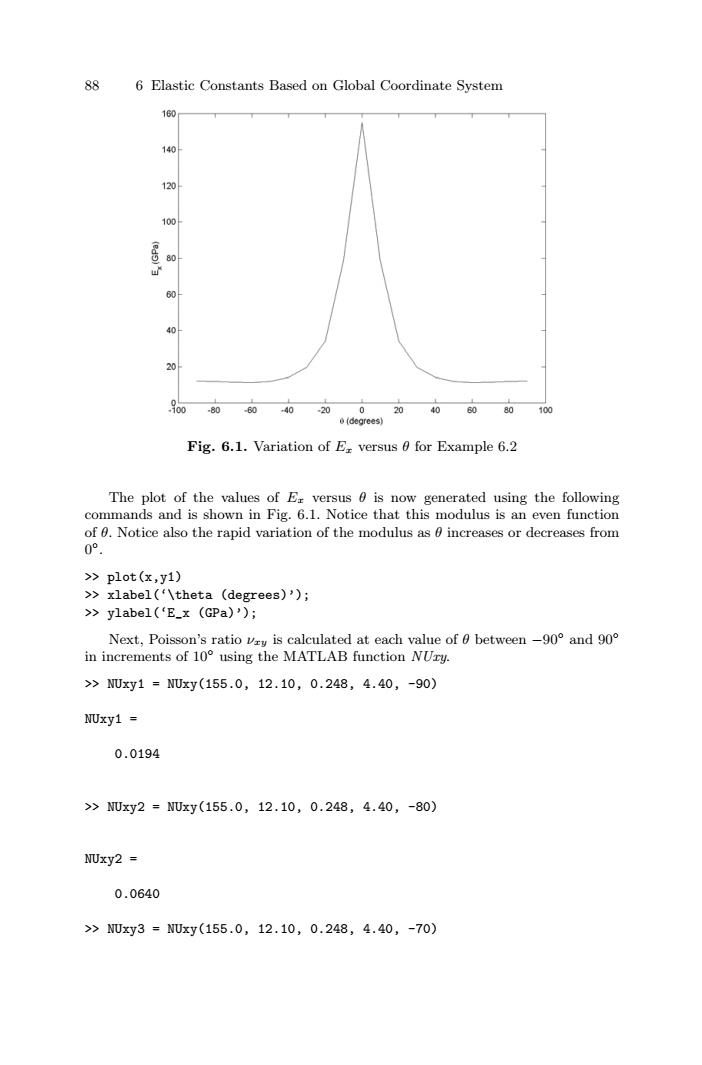
88 6 Elastic Constants Based on Global Coordinate System 760 140 120 100 60 20 80-6040-20020406080100 (degrees) Fig.6.1.Variation of E versus 0 for Example 6.2 The plot of the values of Er versus 0 is now generated using the following commands and is shown in Fig.6.1.Notice that this modulus is an even function of 0.Notice also the rapid variation of the modulus as 0 increases or decreases from 0°. >plot(x,y1) >xlabel('\theta (degrees)'); >ylabel('E_x (GPa)'); Next,Poisson's ratio vry is calculated at each value of 0 between-90 and 90 in increments of 10 using the MATLAB function NUry. >NUxy1=NUxy(155.0,12.10,0.248,4.40,-90) NUxy1 0.0194 >NUxy2=NUxy(155.0,12.10,0.248,4.40,-80) NUxy2 0.0640 >NDxy3=NUxy(155.0,12.10,0.248,4.40,-70)88 6 Elastic Constants Based on Global Coordinate System Fig. 6.1. Variation of Ex versus θ for Example 6.2 The plot of the values of Ex versus θ is now generated using the following commands and is shown in Fig. 6.1. Notice that this modulus is an even function of θ. Notice also the rapid variation of the modulus as θ increases or decreases from 0◦. >> plot(x,y1) >> xlabel(‘\theta (degrees)’); >> ylabel(‘E_x (GPa)’); Next, Poisson’s ratio νxy is calculated at each value of θ between −90◦ and 90◦ in increments of 10◦ using the MATLAB function NUxy. >> NUxy1 = NUxy(155.0, 12.10, 0.248, 4.40, -90) NUxy1 = 0.0194 >> NUxy2 = NUxy(155.0, 12.10, 0.248, 4.40, -80) NUxy2 = 0.0640 >> NUxy3 = NUxy(155.0, 12.10, 0.248, 4.40, -70)