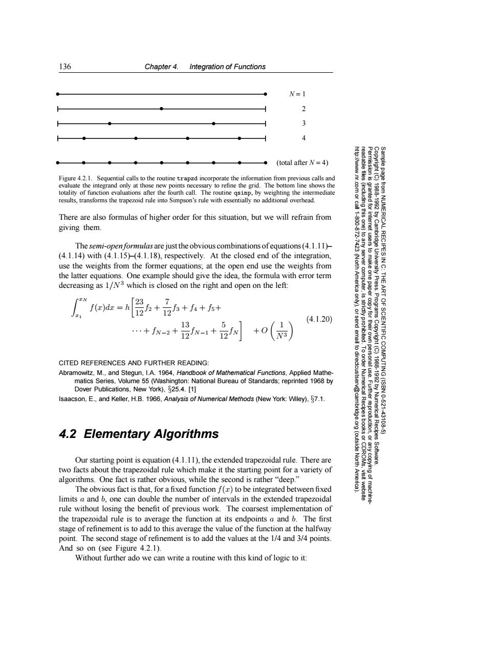
136 Chapter 4.Integration of Functions N=1 2 3 ● 4 ● -●(total after N=4) Figure 4.2.1.Sequential calls to the routine trapzd incorporate the information from previous calls and evaluate the integrand only at those new points necessary to refine the grid.The bottom line shows the totality of function evaluations after the fourth call.The routine gsimp,by weighting the intermediate results,transforms the trapezoid rule into Simpson's rule with essentially no additional overhead. There are also formulas of higher order for this situation,but we will refrain from 以2 giving them. The semi-open formulas are just the obvious combinations ofequations(4.1.11)- RECIPES (4.1.14)with(4.1.15)-(4.1.18),respectively.At the closed end of the integration, b 令 use the weights from the former equations:at the open end use the weights from the latter equations.One example should give the idea,the formula with error term decreasing as 1/N3 which is closed on the right and open on the left: Press. 23 1 fa=h++f+6+ (4.1.20) 13 5 +fN-2+12fN-1+2fN +0(a) 61 CITED REFERENCES AND FURTHER READING: Abramowitz,M.,and Stegun,I.A.1964,Handbook of Mathematical Functions,Applied Mathe- matics Series,Volume 55 (Washington:National Bureau of Standards;reprinted 1968 by Dover Publications,New York),$25.4.[1] Isaacson,E.,and Keller,H.B.1966,Analysis of Numerical Methods(New York:Wiley).$7.1. Numerical Recipes 10.621 E喜 43106 4.2 Elementary Algorithms (outside Our starting point is equation(4.1.11),the extended trapezoidal rule.There are North Software. two facts about the trapezoidal rule which make it the starting point for a variety of algorithms.One fact is rather obvious,while the second is rather"deep." The obvious fact is that,for a fixed function f(z)to be integrated between fixed limits a and b,one can double the number of intervals in the extended trapezoidal rule without losing the benefit of previous work.The coarsest implementation of the trapezoidal rule is to average the function at its endpoints a and b.The first stage of refinement is to add to this average the value of the function at the halfway point.The second stage of refinement is to add the values at the 1/4 and 3/4 points. And so on (see Figure 4.2.1). Without further ado we can write a routine with this kind of logic to it:136 Chapter 4. Integration of Functions Permission is granted for internet users to make one paper copy for their own personal use. Further reproduction, or any copyin Copyright (C) 1988-1992 by Cambridge University Press. Programs Copyright (C) 1988-1992 by Numerical Recipes Software. Sample page from NUMERICAL RECIPES IN C: THE ART OF SCIENTIFIC COMPUTING (ISBN 0-521-43108-5) g of machine￾readable files (including this one) to any server computer, is strictly prohibited. To order Numerical Recipes books or CDROMs, visit website http://www.nr.com or call 1-800-872-7423 (North America only), or send email to directcustserv@cambridge.org (outside North America). N = 1 2 3 4 (total after N = 4) Figure 4.2.1. Sequential calls to the routine trapzd incorporate the information from previous calls and evaluate the integrand only at those new points necessary to refine the grid. The bottom line shows the totality of function evaluations after the fourth call. The routine qsimp, by weighting the intermediate results, transforms the trapezoid rule into Simpson’s rule with essentially no additional overhead. There are also formulas of higher order for this situation, but we will refrain from giving them. The semi-open formulas are just the obvious combinations of equations (4.1.11)– (4.1.14) with (4.1.15)–(4.1.18), respectively. At the closed end of the integration, use the weights from the former equations; at the open end use the weights from the latter equations. One example should give the idea, the formula with error term decreasing as 1/N 3 which is closed on the right and open on the left:
xN x1 f(x)dx = h 23 12f2 + 7 12f3 + f4 + f5+ ··· + fN−2 + 13 12fN−1 + 5 12fN + O  1 N3  (4.1.20) CITED REFERENCES AND FURTHER READING: Abramowitz, M., and Stegun, I.A. 1964, Handbook of Mathematical Functions, Applied Mathe￾matics Series, Volume 55 (Washington: National Bureau of Standards; reprinted 1968 by Dover Publications, New York), §25.4. [1] Isaacson, E., and Keller, H.B. 1966, Analysis of Numerical Methods (New York: Wiley), §7.1. 4.2 Elementary Algorithms Our starting point is equation (4.1.11), the extended trapezoidal rule. There are two facts about the trapezoidal rule which make it the starting point for a variety of algorithms. One fact is rather obvious, while the second is rather “deep.” The obvious fact is that, for a fixed function f(x) to be integrated between fixed limits a and b, one can double the number of intervals in the extended trapezoidal rule without losing the benefit of previous work. The coarsest implementation of the trapezoidal rule is to average the function at its endpoints a and b. The first stage of refinement is to add to this average the value of the function at the halfway point. The second stage of refinement is to add the values at the 1/4 and 3/4 points. And so on (see Figure 4.2.1). Without further ado we can write a routine with this kind of logic to it: