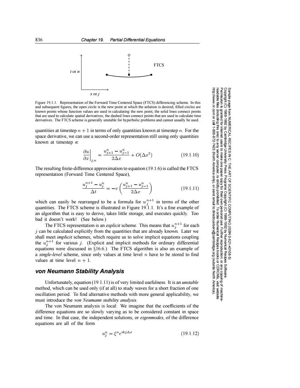
836 Chapter 19.Partial Differential Equations 个 0 FTCS x orj Figure 19.1.1.Representation of the Forward Time Centered Space(FTCS)differencing scheme.In this and subsequent figures,the open circle is the new point at which the solution is desired;filled circles are known points whose function values are used in calculating the new point;the solid lines connect points that are used to calculate spatial derivatives;the dashed lines connect points that are used to calculate time derivatives.The FTCS scheme is generally unstable for hyperbolic problems and cannot usually be used. nted for quantities at timestep n+1 in terms of only quantities known at timestep n.For the space derivative,we can use a second-order representation still using only quantities known at timestep n: Ou 0加 u吲+1-1+0（△x2)） RECIPES (19.1.10) 2△x 令 The resulting finite-difference approximation to equation(19.1.6)is called the FTCS representation (Forward Time Centered Space), ,为 u+1-吗 /u+1-u-1 At (19.1.11) 2△x which can easily be rearranged to be a formula for u+in terms of the other IENTIFIC quantities.The FTCS scheme is illustrated in Figure 19.1.1.It's a fine example of 6 an algorithm that is easy to derive,takes little storage,and executes quickly.Too bad it doesn't work!(See below.) The FTCS representation is an explicit scheme.This means thatfor each jcan be calculated explicitly from the quantities that are already known.Later we shall meet implicit schemes,which require us to solve implicit equations coupling the u for various j.(Explicit and implicit methods for ordinary differential 10.621 equations were discussed in 816.6.)The FTCS algorithm is also an example of a single-level scheme,since only values at time level n have to be stored to find E喜 43106 values at time level n+1. (outside von Neumann Stability Analysis North Software. Unfortunately,equation(19.1.11)is of very limited usefulness.It is an unstable method,which can be used only (if at all)to study waves for a short fraction of one oscillation period.To find alternative methods with more general applicability,we must introduce the von Neumann stability analysis. The von Neumann analysis is local:We imagine that the coefficients of the difference equations are so slowly varying as to be considered constant in space and time.In that case,the independent solutions,or eigenmodes,of the difference equations are all of the form un=gneikjAr (19.1.12)836 Chapter 19. Partial Differential Equations Permission is granted for internet users to make one paper copy for their own personal use. Further reproduction, or any copyin Copyright (C) 1988-1992 by Cambridge University Press. Programs Copyright (C) 1988-1992 by Numerical Recipes Software. Sample page from NUMERICAL RECIPES IN C: THE ART OF SCIENTIFIC COMPUTING (ISBN 0-521-43108-5) g of machine￾readable files (including this one) to any server computer, is strictly prohibited. To order Numerical Recipes books or CDROMs, visit website http://www.nr.com or call 1-800-872-7423 (North America only), or send email to directcustserv@cambridge.org (outside North America). t or n x or j FTCS Figure 19.1.1. Representation of the Forward Time Centered Space (FTCS) differencing scheme. In this and subsequent figures, the open circle is the new point at which the solution is desired; filled circles are known points whose function values are used in calculating the new point; the solid lines connect points that are used to calculate spatial derivatives; the dashed lines connect points that are used to calculate time derivatives. The FTCS scheme is generally unstable for hyperbolic problems and cannot usually be used. quantities at timestep n + 1 in terms of only quantities known at timestep n. For the space derivative, we can use a second-order representation still using only quantities known at timestep n: ∂u ∂x j,n = un j+1 − un j−1 2∆x + O(∆x2) (19.1.10) The resulting finite-difference approximation to equation (19.1.6) is called the FTCS representation (Forward Time Centered Space), un+1 j − un j ∆t = −v
un j+1 − un j−1 2∆x (19.1.11) which can easily be rearranged to be a formula for u n+1 j in terms of the other quantities. The FTCS scheme is illustrated in Figure 19.1.1. It’s a fine example of an algorithm that is easy to derive, takes little storage, and executes quickly. Too bad it doesn’t work! (See below.) The FTCS representation is an explicit scheme. This means that un+1 j for each j can be calculated explicitly from the quantities that are already known. Later we shall meet implicit schemes, which require us to solve implicit equations coupling the un+1 j for various j. (Explicit and implicit methods for ordinary differential equations were discussed in §16.6.) The FTCS algorithm is also an example of a single-level scheme, since only values at time level n have to be stored to find values at time level n + 1. von Neumann Stability Analysis Unfortunately, equation (19.1.11) is of very limited usefulness. It is an unstable method, which can be used only (if at all) to study waves for a short fraction of one oscillation period. To find alternative methods with more general applicability, we must introduce the von Neumann stability analysis. The von Neumann analysis is local: We imagine that the coefficients of the difference equations are so slowly varying as to be considered constant in space and time. In that case, the independent solutions, or eigenmodes, of the difference equations are all of the form un j = ξneikj∆x (19.1.12)