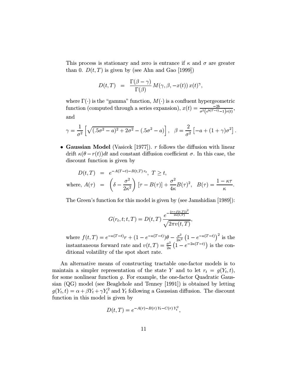
This process is stationary and zero is entrance if K and o are greater than 0.D(t,T)is given by (see Ahn and Gao 1999]) Dk,=IT32M,日，-e)z0, T() where I()is the "gamma"function,M()is a confluent hypergeometric function (computed through a series expansion),() .2h and [VGo-aP+2g-(52-小，月-2[-a+1+. 1 y=1 Gaussian Model (Vasicek [1977).r follows the diffusion with linear drift (-r(t))dt and constant diffusion coefficient o.In this case,the discount function is given by D(t,T)= eA(T-t-Bt,T),T≥t, where,A(r) 2 6-aol+8G,0)-1 The Green's function for this model is given by (see Jamshidian [1989): r-6①2 2(t,1) G（rt,t:t,T)=D(t,T) V27v(t,T where f(化，T)=eT-r+(1-e-*T-)0-茶(1-eT-)2 is the instantaneous forward rate and (t,T)(1-e()is the con- ditional volatility of the spot short rate. An alternative means of constructing tractable one-factor models is to maintain a simpler representation of the state Y and to let rt=g(Yi,t), for some nonlinear function g.For example,the one-factor Quadratic Gaus- sian (QG)model (see Beaglehole and Tenney [1991])is obtained by letting g(Yi,t)=a+BY+Y2 and Yi following a Gaussian diffusion.The discount function in this model is given by D化，T)=eA()-B(r)-C)竖. 11This process is stationary and zero is entrance if κ and σ are greater than 0. D(t, T) is given by (see Ahn and Gao [1999]) D(t, T) = Γ(β − γ) Γ(β) M(γ, β, −x(t)) x(t) γ , where Γ(·) is the “gamma” function, M(·) is a confluent hypergeometric function (computed through a series expansion), x(t) = −2b σ2(eb(T−t)−1)r(t) , and γ = 1 σ2 hp(.5σ2 − a)2 + 2σ2 − (.5σ2 − a) i , β = 2 σ2 −a + (1 + γ)σ2 . • Gaussian Model (Vasicek [1977]). r follows the diffusion with linear drift κ(θ −r(t))dt and constant diffusion coefficient σ. In this case, the discount function is given by D(t, T) = e−A(T −t)−B(t,T) rt , T ≥ t, where, A(τ ) =  δ − σ2 2κ2  [τ − B(τ )] + σ2 4κ B(τ ) 2 , B(τ ) = 1 − κτ κ . The Green’s function for this model is given by (see Jamshidian [1989]): G(rt, t;t, T) = D(t, T) e − (r−f(t,T ))2 2v(t,T ) p2πv(t, T) , where f(t, T) = e−κ(T −t) r + (1 − e−κ(T −t) )θ − σ2 2κ2 ￾ 1 − e−κ(T −t)
2 is the instantaneous forward rate and v(t, T) = σ2 2κ ￾ 1 − e−2κ(T −t)
is the con￾ditional volatility of the spot short rate. An alternative means of constructing tractable one-factor models is to maintain a simpler representation of the state Y and to let rt = g(Yt, t), for some nonlinear function g. For example, the one-factor Quadratic Gaus￾sian (QG) model (see Beaglehole and Tenney [1991]) is obtained by letting g(Yt, t) = α + βYt + γY 2 t and Yt following a Gaussian diffusion. The discount function in this model is given by D(t, T) = e−A(τ)−B(τ) Yt−C(τ) Y 2 t , 11