正在加载图片...

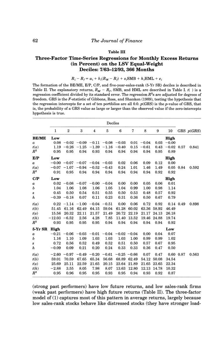
62 The Journal of Finance Table IⅡ Three-Factor Time-Series Regressions for Monthly Excess Returns (in Percent)on the LSV Equal-Weight Deciles:7/63-12/93,366 Months Ri-R=ai+b:(RM-R+s SMB+h;HML+e; The formation of the BE/ME,E/P,C/P,and five-year-sales-rank (5-Yr SR)deciles is described in Table II.The explanatory returns,R-R,SMB,and HML are described in Table I.t()is a regression coefficient divided by its standard error.The regression R2s are adjusted for degrees of freedom.GRS is the F-statistic of Gibbons,Ross,and Shanken(1989),testing the hypothesis that the regression intercepts for a set of ten portfolios are all 0.0.p(GRS)is the p-value of GRS,that is,the probability of a GRS value as large or larger than the observed value if the zero-intercepts hypothesis is true. Deciles 1 3 4 5 6 7 8 9 10 GRS D(GRS) BE/ME Low High 令 0.08 -0.02 -0.09 -0.11-0.08 -0.03 0.01-0.040.03 -0.00 ) 1.19 -0.26 -1.25 -1.39 -1.16-0.40 0.15-0.61 0.43 -0.020.570.841 R2 0.95 0.95 0.94 0.93 0.940.94 0.940.940.95 0.89 EP Low High a -0.00-0.07 -0.07-0.04-0.03 0.020.06 0.090.12 0.00 ta) -0.07-1.07 -0.94-0.52-0.43 0.241.01 1.461.49 0.050.840.592 R2 0.91 0.95 0.94 0.94 0.94 0.940.94 0.940.92 0.92 C/P Low High 0.02-0.08 -0.07-0.00 -0.04 0.000.00 0.050.060.01 b 1.04 1.06 1.08 1.06 1.05 1.04 0.99 1.000.98 1.14 0.45 0.50 0.54 0.51 0.55 0.50 0.53 0.48 0.57 0.92 b -0.39-0.18 0.07 0.11 0.23 0.310.36 0.500.67 0.79 t(a) 0.22-1.14-1.00 -0.04 -0.51 0.00 0.06 0.720.92 0.140.49 0.898 t(b) 51.4561.1662.4964.1559.04 61.2860.0263.3658.92 46.49 t(s) 15.5620.3222.1121.5721.4920.7222.1921.1724.1326.18 t(h) -12.03 -6.52 2.564.28 7.8511.4013.5219.4624.8819.74 R2 0.93 0.95 0.95 0.95 0.94 0.940.94 0.940.94 0.92 5-Yr SR High Low -0.21 -0.06 -0.03-0.01 -0.04 -0.02-0.04 0.000.04 0.07 6 1.16 1.10 1.09 1.03 1.03 1.031.00 0.99 0.99 1.02 0.72 0.56 0.52 0.49 0.52 0.510.500.570.67 0.95 h -0.09 0.09 0.21 0.20 0.24 0.330.33 0.36 0.47 0.50 t(a) -2.60-0.97-0.49-0.20-0.61-0.25-0.660.070.47 0.600.870.563 t(b) 59.0170.5967.6565.3456.6868.8962.4954.1250.0834.54 t(s) 25.6925.1122.5921.6520.1523.6421.8921.6523.6522.34 t(h) -2.88 3.55 8.057.98 8.0713.6312.8012.1314.7810.32 R2 0.950.960.950.950.930.950.940.930.920.87 (strong past performers)have low future returns,and low sales-rank firms (weak past performers)have high future returns(Table II).The three-factor model of(1)captures most of this pattern in average returns,largely because low sales-rank stocks behave like distressed stocks (they have stronger load-