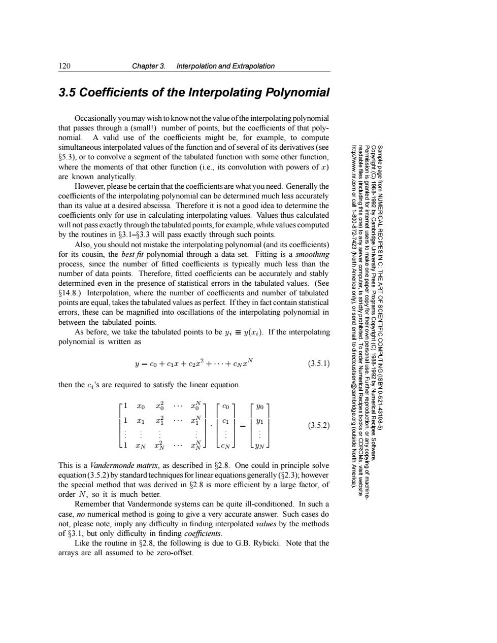
120 Chapter 3.Interpolation and Extrapolation 3.5 Coefficients of the Interpolating Polynomial Occasionally you may wish to know not the value of the interpolating polynomial that passes through a (small!)number of points,but the coefficients of that poly- nomial.A valid use of the coefficients might be,for example,to compute simultaneous interpolated values of the function and of several of its derivatives (see S5.3),or to convolve a segment of the tabulated function with some other function, where the moments of that other function (i.e..its convolution with powers of x) are known analytically. However,please be certain that the coefficients are what you need.Generally the coefficients of the interpolating polynomial can be determined much less accurately than its value at a desired abscissa.Therefore it is not a good idea to determine the coefficients only for use in calculating interpolating values.Values thus calculated will not pass exactly through the tabulated points,for example,while values computed by the routines in 83.1-83.3 will pass exactly through such points. Also,you should not mistake the interpolating polynomial(and its coefficients) for its cousin,the best fit polynomial through a data set.Fitting is a smoothing 2 process,since the number of fitted coefficients is typically much less than the number of data points.Therefore,fitted coefficients can be accurately and stably determined even in the presence of statistical errors in the tabulated values.(See $14.8.)Interpolation,where the number of coefficients and number of tabulated points are equal,takes the tabulated values as perfect.If they in fact contain statistical errors,these can be magnified into oscillations of the interpolating polynomial in 其色% between the tabulated points. As before,we take the tabulated points to be yi=y(i).If the interpolating OF SCIENTIFIC( polynomial is written as 61 y=co+ci+c22+...+CNzN (3.5.1) then the ci's are required to satisfy the linear equation 1 To 哈 C07 yo Numerica 10.621 1 x 1 431 (3.5.2) (outside Recipes TN CN -yN North This is a Vandermonde matrix,as described in $2.8.One could in principle solve equation(3.5.2)by standard techniques for linear equations generally(82.3);however the special method that was derived in 82.8 is more efficient by a large factor,of order N,so it is much better. Remember that Vandermonde systems can be quite ill-conditioned.In such a case,no numerical method is going to give a very accurate answer.Such cases do not,please note,imply any difficulty in finding interpolated values by the methods of 83.1,but only difficulty in finding coefficients. Like the routine in $2.8,the following is due to G.B.Rybicki.Note that the arrays are all assumed to be zero-offset.120 Chapter 3. Interpolation and Extrapolation Permission is granted for internet users to make one paper copy for their own personal use. Further reproduction, or any copyin Copyright (C) 1988-1992 by Cambridge University Press. Programs Copyright (C) 1988-1992 by Numerical Recipes Software. Sample page from NUMERICAL RECIPES IN C: THE ART OF SCIENTIFIC COMPUTING (ISBN 0-521-43108-5) g of machine￾readable files (including this one) to any server computer, is strictly prohibited. To order Numerical Recipes books or CDROMs, visit website http://www.nr.com or call 1-800-872-7423 (North America only), or send email to directcustserv@cambridge.org (outside North America). 3.5 Coefficients of the Interpolating Polynomial Occasionally you may wish to know not the value of the interpolating polynomial that passes through a (small!) number of points, but the coefficients of that poly￾nomial. A valid use of the coefficients might be, for example, to compute simultaneous interpolated values of the function and of several of its derivatives (see §5.3), or to convolve a segment of the tabulated function with some other function, where the moments of that other function (i.e., its convolution with powers of x) are known analytically. However, please be certain that the coefficients are what you need. Generally the coefficients of the interpolating polynomial can be determined much less accurately than its value at a desired abscissa. Therefore it is not a good idea to determine the coefficients only for use in calculating interpolating values. Values thus calculated will not pass exactly through the tabulated points,for example, while values computed by the routines in §3.1–§3.3 will pass exactly through such points. Also, you should not mistake the interpolating polynomial (and its coefficients) for its cousin, the best fit polynomial through a data set. Fitting is a smoothing process, since the number of fitted coefficients is typically much less than the number of data points. Therefore, fitted coefficients can be accurately and stably determined even in the presence of statistical errors in the tabulated values. (See §14.8.) Interpolation, where the number of coefficients and number of tabulated points are equal, takes the tabulated values as perfect. If they in fact contain statistical errors, these can be magnified into oscillations of the interpolating polynomial in between the tabulated points. As before, we take the tabulated points to be yi ≡ y(xi). If the interpolating polynomial is written as y = c0 + c1x + c2x2 + ··· + cN xN (3.5.1) then the ci’s are required to satisfy the linear equation      1 x0 x2 0 ··· xN 0 1 x1 x2 1 ··· xN 1 . . . . . . . . . . . . 1 xN x2 N ··· xN N      ·      c0 c1 . . . cN      =      y0 y1 . . . yN      (3.5.2) This is a Vandermonde matrix, as described in §2.8. One could in principle solve equation (3.5.2) by standard techniques for linear equations generally (§2.3); however the special method that was derived in §2.8 is more efficient by a large factor, of order N, so it is much better. Remember that Vandermonde systems can be quite ill-conditioned. In such a case, no numerical method is going to give a very accurate answer. Such cases do not, please note, imply any difficulty in finding interpolated values by the methods of §3.1, but only difficulty in finding coefficients. Like the routine in §2.8, the following is due to G.B. Rybicki. Note that the arrays are all assumed to be zero-offset