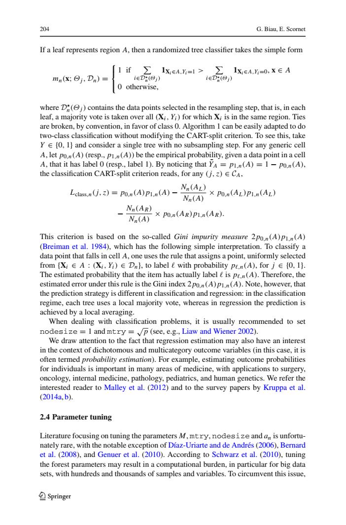
204 G.Biau,E.Scornet If a leaf represents region A,then a randomized tree classifier takes the simple form if ∑1xeA.y,=> ∑1xeA,Y=0,X∈A mn(X;⊙j,Dn) ieD(⊙j) ieD:(ej) 0 otherwise, where D"(;)contains the data points selected in the resampling step,that is,in each leaf,a majority vote is taken over all (Xi,Yi)for which Xi is in the same region.Ties are broken,by convention,in favor of class 0.Algorithm 1 can be easily adapted to do two-class classification without modifying the CART-split criterion.To see this,take Y E(0,1)and consider a single tree with no subsampling step.For any generic cell A,let po.n(A)(resp.,pin(A))be the empirical probability,given a data point in a cell A,that it has label 0 (resp.,label 1).By noticing that YA =pi.n(A)=1-po.n(A). the classification CART-split criterion reads,for any (j,z)ECA, Lcassn(j)=po(A)p(A)-N(AL) Nn(A) ×P0,n(AL)P1.n(AL) Nn(AR) ×p0.n(AR)p1,n(AR). Nn(A) This criterion is based on the so-called Gini impurity measure 2po.n(A)pi.n(A) (Breiman et al.1984),which has the following simple interpretation.To classify a data point that falls in cell A,one uses the rule that assigns a point,uniformly selected from{X∈A:(X,Yi)∈Dn,to label e with probability pe.n(A),forj∈{0，l. The estimated probability that the item has actually label e is pe.n(A).Therefore,the estimated error under this rule is the Gini index 2po.n(A)pI.n(A).Note,however,that the prediction strategy is different in classification and regression:in the classification regime,each tree uses a local majority vote,whereas in regression the prediction is achieved by a local averaging. When dealing with classification problems,it is usually recommended to set nodesize 1 and mtry =p(see,e.g.,Liaw and Wiener 2002). We draw attention to the fact that regression estimation may also have an interest in the context of dichotomous and multicategory outcome variables (in this case,it is often termed probability estimation).For example,estimating outcome probabilities for individuals is important in many areas of medicine,with applications to surgery, oncology,internal medicine,pathology,pediatrics,and human genetics.We refer the interested reader to Malley et al.(2012)and to the survey papers by Kruppa et al. 2014a,b). 2.4 Parameter tuning Literature focusing on tuning the parameters M,mtry,nodesize and an is unfortu- nately rare,with the notable exception of Diaz-Uriarte and de Andres(2006),Bernard et al.(2008),and Genuer et al.(2010).According to Schwarz et al.(2010),tuning the forest parameters may result in a computational burden,in particular for big data sets,with hundreds and thousands of samples and variables.To circumvent this issue, Springer204 G. Biau, E. Scornet If a leaf represents region A, then a randomized tree classifier takes the simple form mn(x; Θj, Dn) = ⎧ ⎨ ⎩ 1 if  i∈D n (Θj) 1Xi∈A,Yi=1 >  i∈D n (Θj) 1Xi∈A,Yi=0, x ∈ A 0 otherwise, where D n(Θj) contains the data points selected in the resampling step, that is, in each leaf, a majority vote is taken over all (Xi, Yi) for which Xi is in the same region. Ties are broken, by convention, in favor of class 0. Algorithm 1 can be easily adapted to do two-class classification without modifying the CART-split criterion. To see this, take Y ∈ {0, 1} and consider a single tree with no subsampling step. For any generic cell A, let p0,n(A) (resp., p1,n(A)) be the empirical probability, given a data point in a cell A, that it has label 0 (resp., label 1). By noticing that Y¯A = p1,n(A) = 1 − p0,n(A), the classification CART-split criterion reads, for any (j,z) ∈ CA, Lclass,n(j,z) = p0,n(A)p1,n(A) − Nn(AL ) Nn(A) × p0,n(AL )p1,n(AL ) − Nn(AR) Nn(A) × p0,n(AR)p1,n(AR). This criterion is based on the so-called Gini impurity measure 2p0,n(A)p1,n(A) (Breiman et al. 1984), which has the following simple interpretation. To classify a data point that falls in cell A, one uses the rule that assigns a point, uniformly selected from {Xi ∈ A : (Xi, Yi) ∈ Dn}, to label  with probability p,n(A), for j ∈ {0, 1}. The estimated probability that the item has actually label  is p,n(A). Therefore, the estimated error under this rule is the Gini index 2p0,n(A)p1,n(A). Note, however, that the prediction strategy is different in classification and regression: in the classification regime, each tree uses a local majority vote, whereas in regression the prediction is achieved by a local averaging. When dealing with classification problems, it is usually recommended to set nodesize = 1 and mtry = √p (see, e.g., Liaw and Wiener 2002). We draw attention to the fact that regression estimation may also have an interest in the context of dichotomous and multicategory outcome variables (in this case, it is often termed probability estimation). For example, estimating outcome probabilities for individuals is important in many areas of medicine, with applications to surgery, oncology, internal medicine, pathology, pediatrics, and human genetics. We refer the interested reader to Malley et al. (2012) and to the survey papers by Kruppa et al. (2014a, b). 2.4 Parameter tuning Literature focusing on tuning the parameters M, mtry, nodesize and an is unfortu￾nately rare, with the notable exception of Díaz-Uriarte and de Andrés (2006), Bernard et al. (2008), and Genuer et al. (2010). According to Schwarz et al. (2010), tuning the forest parameters may result in a computational burden, in particular for big data sets, with hundreds and thousands of samples and variables. To circumvent this issue, 123