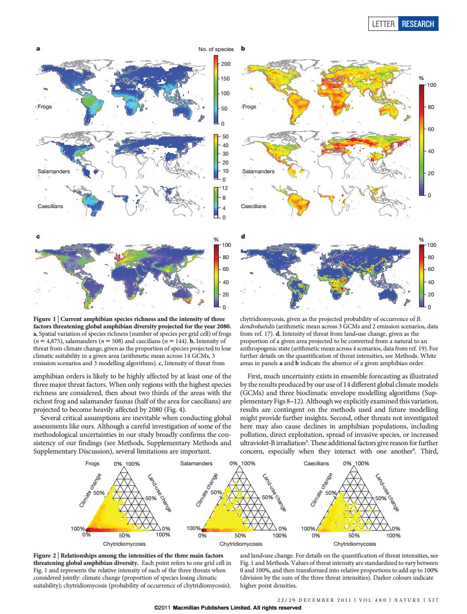
LETTER RESEARCH No.of species 200 150 % 100 100 Frogs 80 0 60 50 6000 40 10 Salamanders 20 0 % 100 100 80 60 40 0 20 0 0 Figure 1 Current amphibian species richness and the intensity of three chytridiomycosis,given as the projected probability of occurrence of B. factors threatening global amphibian diversity projected for the year 2080 dendrobatidis (arithmetic mean across 3 GCMs and 2 emission scenarios,data a,Spatial variation of species richness(number of species per grid cell)of frogs from ref.17).d,Intensity of threat from land-use change,given as the (n 4,875),salamanders (n 508)and caecilians (n=144).b,Intensity of proportion of a given area projected to be converted from a natural to an threat from climate change,given as the proportion of species projected to lose anthropogenic state(arithmetic mean across 4 scenarios,data from ref.19).For climatic suitability in a given area(arithmetic mean across 14 GCMs,3 further details on the quantification of threat intensities,see Methods.White emission scenarios and 3 modelling algorithms).c,Intensity of threat from areas in panels a and b indicate the absence of a given amphibian order. amphibian orders is likely to be highly affected by at least one of the First,much uncertainty exists in ensemble forecasting as illustrated three major threat factors.When only regions with the highest species by the results produced by our use of 14 different global climate models richness are considered,then about two thirds of the areas with the (GCMs)and three bioclimatic envelope modelling algorithms (Sup richest frog and salamander faunas (half of the area for caecilians)are plementary Figs 8-12).Although we explicitly examined this variation, projected to become heavily affected by 2080(Fig.4). results are contingent on the methods used and future modelling Several critical assumptions are inevitable when conducting global might provide further insights.Second,other threats not investigated assessments like ours.Although a careful investigation of some of the here may also cause declines in amphibian populations,including methodological uncertainties in our study broadly confirms the con- pollution,direct exploitation,spread of invasive species,or increased sistency of our findings(see Methods,Supplementary Methods and ultraviolet-B irradiation.These additional factors give reason for further Supplementary Discussion),several limitations are important. concern,especially when they interact with one another.Third, Frogs 0%,100% Salamanders 0%,100% Caecilians 0%100% ge ch 50% 0% nate 50% 509% 100 100% 0% 100% 0% 0% 50% 100% 0% 50% 100% 0% 50% 100% Chytridiomycosis Chytridiomycosis Chytridiomycosis Figure 2 Relationships among the intensities of the three main factors and land-use change.For details on the quantification of threat intensities,see threatening global amphibian diversity.Each point refers to one grid cell in Fig.I and Methods.Values of threat intensity are standardized to vary between Fig.I and represents the relative intensity of each of the three threats when 0 and 100%,and then transformed into relative proportions to add up to 100% considered jointly:climate change(proportion of species losing climatic (division by the sum of the three threat intensities).Darker colours indicate suitability);chytridiomycosis(probability of occurrence of chytridiomycosis); higher point densities. 22/29 DECEMBER 2011 VOL 480I NATURE 517 2011 Macmillan Publishers Limited.All rights reservedamphibian orders is likely to be highly affected by at least one of the three major threat factors. When only regions with the highest species richness are considered, then about two thirds of the areas with the richest frog and salamander faunas (half of the area for caecilians) are projected to become heavily affected by 2080 (Fig. 4). Several critical assumptions are inevitable when conducting global assessments like ours. Although a careful investigation of some of the methodological uncertainties in our study broadly confirms the con￾sistency of our findings (see Methods, Supplementary Methods and Supplementary Discussion), several limitations are important. First, much uncertainty exists in ensemble forecasting as illustrated by the results produced by our use of 14 different global climate models (GCMs) and three bioclimatic envelope modelling algorithms (Sup￾plementary Figs 8–12). Although we explicitly examined this variation, results are contingent on the methods used and future modelling might provide further insights. Second, other threats not investigated here may also cause declines in amphibian populations, including pollution, direct exploitation, spread of invasive species, or increased ultraviolet-B irradiation5 . These additional factors give reason for further concern, especially when they interact with one another4 . Third, Frogs Salamanders Caecilians b c d 0 10 20 30 40 50 0 4 8 12 50 100 150 200 0 No. of species Frogs Salamanders Caecilians a 0 20 40 60 80 100 % 0 20 40 60 80 100 % 0 20 40 60 80 100 % Figure 1 | Current amphibian species richness and the intensity of three factors threatening global amphibian diversity projected for the year 2080. a, Spatial variation of species richness (number of species per grid cell) of frogs (n 5 4,875), salamanders (n 5 508) and caecilians (n 5 144). b, Intensity of threat from climate change, given as the proportion of species projected to lose climatic suitability in a given area (arithmetic mean across 14 GCMs, 3 emission scenarios and 3 modelling algorithms). c, Intensity of threat from chytridiomycosis, given as the projected probability of occurrence of B. dendrobatidis (arithmetic mean across 3 GCMs and 2 emission scenarios, data from ref. 17). d, Intensity of threat from land-use change, given as the proportion of a given area projected to be converted from a natural to an anthropogenic state (arithmetic mean across 4 scenarios, data from ref. 19). For further details on the quantification of threat intensities, see Methods. White areas in panels a and b indicate the absence of a given amphibian order. Chytridiomycosis 0% 100% Climate change 100% 0% 100% 0% Land-use change 50% 50% 50% Chytridiomycosis 0% 100% Climate change 100% 0% 100% 0% Land-use change 50% 50% 50% Frogs Salamanders Caecilians Chytridiomycosis 0% 100% Climate change 100% 0% 100% 0% Land-use change 50% 50% 50% Figure 2 | Relationships among the intensities of the three main factors threatening global amphibian diversity. Each point refers to one grid cell in Fig. 1 and represents the relative intensity of each of the three threats when considered jointly: climate change (proportion of species losing climatic suitability); chytridiomycosis (probability of occurrence of chytridiomycosis); and land-use change. For details on the quantification of threat intensities, see Fig. 1 and Methods. Values of threat intensity are standardized to vary between 0 and 100%, and then transformed into relative proportions to add up to 100% (division by the sum of the three threat intensities). Darker colours indicate higher point densities. LETTER RESEARCH 22/29 DECEMBER 2011 | VOL 480 | NATURE | 517 ©2011 Macmillan Publishers Limited. All rights reserved