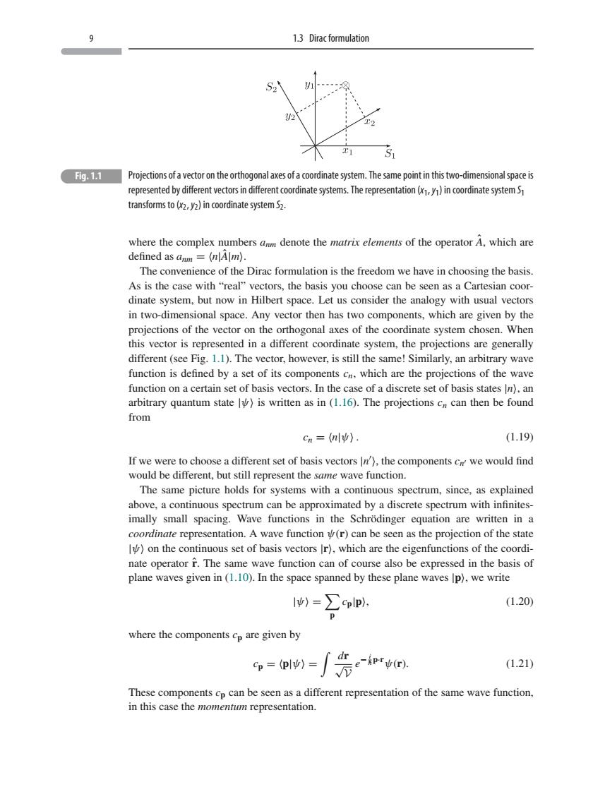
1.3 Diracformulation Projections of a vector on the orthogonal axes of a coordinate system.The same point in this two-dimensional space is represented by differntvectors indifferentrdate systems.The representation(inrdinate systemS where the complex numbers anm denote the matrix elements of the operator A,which are defined as anm =(nlAlm). The conve ience of the Dirac formulation is the freedom we have in choosing the basis. As is the case with"real"ve tors,the basis you choose can be seen as a Cartesian coo dinate system,but now in Hilbert space.Let us consider the analogy with usual vectors in two-dimensional space.Any vector then has two components,which are given by the projections of the vector on the orthogonal axes of the coordinate system chosen.When this vector is represented in a different coordinate system,the projections are generally different(see Fig.1.1).The vector,however,is still th me!Smilarly,rbitrary wave function is defined by a set of its are the projections of the wave function on a certain set of basis vectors.In the case of a discrete set of basis states In),an arbitrary quantum state)is written as in(1.16).The projections cn can then be found from cn=川) (1.19 If we were to choose a different set of basis vectors n).the components c we would find would be different,but still represent the same wave function. The same picture holds for systems with a continuous spectrum,since,as explained above,a continuous spectrum can be approximated by a discrete spectrum with infinites- imally small spacing.Wave functions in the Schrodinger equation are written in a coordinate representation.A wave function)can be seen as the projection of the stat v)on the continuous set of basis vectors r).which are the eigenfunctions of the coordi nate operator f.The same wave function can of course also be expressed in the basis of plane waves given in (1.10).In the space spanned by these plane waves Ip),we write w)=∑cplp (1.20) where the components cp are given by Cp =(plv)= (1.21) These components cp can be seen as a different representation of the same wave function. in this case the ntation 9 1.3 Dirac formulation Fig. 1.1 Projections of a vector on the orthogonal axes of a coordinate system. The same point in this two-dimensional space is represented by different vectors in different coordinate systems. The representation (x1,y1) in coordinate system S1 transforms to (x2,y2) in coordinate system S2. where the complex numbers anm denote the matrix elements of the operator Aˆ, which are defined as anm = n|Aˆ|m. The convenience of the Dirac formulation is the freedom we have in choosing the basis. As is the case with “real” vectors, the basis you choose can be seen as a Cartesian coor￾dinate system, but now in Hilbert space. Let us consider the analogy with usual vectors in two-dimensional space. Any vector then has two components, which are given by the projections of the vector on the orthogonal axes of the coordinate system chosen. When this vector is represented in a different coordinate system, the projections are generally different (see Fig. 1.1). The vector, however, is still the same! Similarly, an arbitrary wave function is defined by a set of its components cn, which are the projections of the wave function on a certain set of basis vectors. In the case of a discrete set of basis states |n, an arbitrary quantum state |ψ is written as in (1.16). The projections cn can then be found from cn = n|ψ. (1.19) If we were to choose a different set of basis vectors |n , the components cn we would find would be different, but still represent the same wave function. The same picture holds for systems with a continuous spectrum, since, as explained above, a continuous spectrum can be approximated by a discrete spectrum with infinites￾imally small spacing. Wave functions in the Schrödinger equation are written in a coordinate representation. A wave function ψ(r) can be seen as the projection of the state |ψ on the continuous set of basis vectors |r, which are the eigenfunctions of the coordi￾nate operator rˆ. The same wave function can of course also be expressed in the basis of plane waves given in (1.10). In the space spanned by these plane waves |p, we write |ψ =  p cp|p, (1.20) where the components cp are given by cp = p|ψ = dr √ V e − i h¯ p·r ψ(r). (1.21) These components cp can be seen as a different representation of the same wave function, in this case the momentum representation.