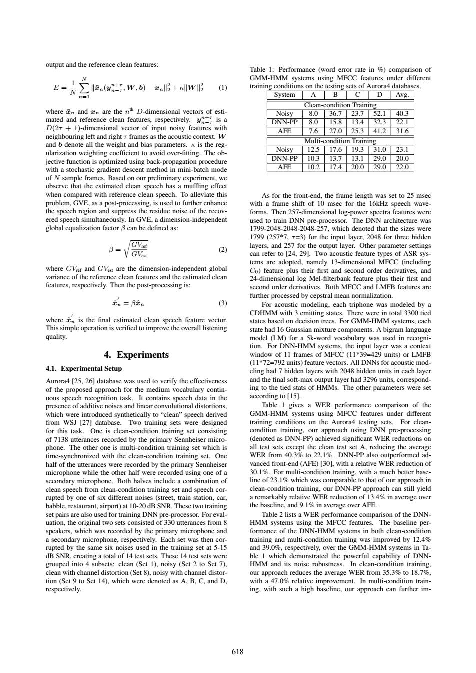
output and the reference clean features: Table 1:Performance (word error rate in %comparison of GMM-HMM systems using MFCC features under different E= 六∑2.(r,w,-x6+wI (1) training conditions on the testing sets of Aurora4 databases. System A D Avg. Clean-condition Training where and n are the nth D-dimensional vectors of esti- Noisy 8.036.723.752.140.3 mated and reference clean features,respectively.is a DNN-PP 8.0 15.813.432.322.1 D(2r+1)-dimensional vector of input noisy features with AFE 7.627.025.341.231.6 neighbouring left and right r frames as the acoustic context.W and b denote all the weight and bias parameters.K is the reg- Multi-condition Training ularization weighting coefficient to avoid over-fitting.The ob- Noisy 12.517.619.331.023.1 jective function is optimized using back-propagation procedure DNN-Pp10.313.713.129.020.0 with a stochastic gradient descent method in mini-batch mode AFE 10.217.420.029.022.0 of N sample frames.Based on our preliminary experiment,we observe that the estimated clean speech has a muffling effect when compared with reference clean speech.To alleviate this As for the front-end,the frame length was set to 25 msec problem,GVE,as a post-processing,is used to further enhance with a frame shift of 10 msec for the 16kHz speech wave- the speech region and suppress the residue noise of the recov- forms.Then 257-dimensional log-power spectra features were ered speech simultaneously.In GVE.a dimension-independent used to train DNN pre-processor.The DNN architecture was global equalization factor B can be defined as 1799-2048-2048-2048-257,which denoted that the sizes were 1799(257*7,T=3)for the input layer,2048 for three hidden GViet B=√GVa (2) layers,and 257 for the output layer.Other parameter settings can refer to [24,29].Two acoustic feature types of ASR sys- tems are adopted,namely 13-dimensional MFCC (including where GVier and GVst are the dimension-independent global Co)feature plus their first and second order derivatives,and variance of the reference clean features and the estimated clean 24-dimensional log Mel-filterbank feature plus their first and features,respectively.Then the post-processing is: second order derivatives.Both MFCC and LMFB features are further processed by cepstral mean normalization 在n=B远 (3) For acoustic modeling,each triphone was modeled by a CDHMM with 3 emitting states.There were in total 3300 tied where is the final estimated clean speech feature vector. states based on decision trees.For GMM-HMM systems,each This simple operation is verified to improve the overall listening state had 16 Gaussian mixture components.A bigram language quality. model (LM)for a 5k-word vocabulary was used in recogni tion.For DNN-HMM systems,the input layer was a context 4.Experiments window of 11 frames of MFCC (11*39=429 units)or LMFB (11*72=792 units)feature vectors.All DNNs for acoustic mod- 4.1.Experimental Setup eling had 7 hidden layers with 2048 hidden units in each layer Aurora4 [25,26]database was used to verify the effectiveness and the final soft-max output layer had 3296 units,correspond- of the proposed approach for the medium vocabulary contin- ing to the tied stats of HMMs.The other parameters were set uous speech recognition task.It contains speech data in the according to [15]. presence of additive noises and linear convolutional distortions. Table 1 gives a WER performance comparison of the which were introduced synthetically to "clean"speech derived GMM-HMM systems using MFCC features under different from WSJ [27]database.Two training sets were designed training conditions on the Aurora4 testing sets.For clean- for this task.One is clean-condition training set consisting condition training,our approach using DNN pre-processing of 7138 utterances recorded by the primary Sennheiser micro- (denoted as DNN-PP)achieved significant WER reductions on phone.The other one is multi-condition training set which is all test sets except the clean test set A,reducing the average time-synchronized with the clean-condition training set.One WER from 40.3%to 22.1%.DNN-PP also outperformed ad- half of the utterances were recorded by the primary Sennheiser vanced front-end (AFE)[30],with a relative WER reduction of microphone while the other half were recorded using one of a 30.1%.For multi-condition training,with a much better base- secondary microphone.Both halves include a combination of line of 23.1%which was comparable to that of our approach in clean speech from clean-condition training set and speech cor- clean-condition training,our DNN-PP approach can still yield rupted by one of six different noises (street,train station,car, a remarkably relative WER reduction of 13.4%in average over babble,restaurant,airport)at 10-20 dB SNR.These two training the baseline,and 9.1%in average over AFE. set pairs are also used for training DNN pre-processor.For eval- Table 2 lists a WER performance comparison of the DNN- uation,the original two sets consisted of 330 utterances from 8 HMM systems using the MFCC features.The baseline per- speakers,which was recorded by the primary microphone and formance of the DNN-HMM systems in both clean-condition a secondary microphone,respectively.Each set was then cor- training and multi-condition training was improved by 12.4% rupted by the same six noises used in the training set at 5-15 and 39.0%,respectively,over the GMM-HMM systems in Ta- dB SNR,creating a total of 14 test sets.These 14 test sets were ble 1 which demonstrated the powerful capability of DNN- grouped into 4 subsets:clean (Set 1),noisy (Set 2 to Set 7) HMM and its noise robustness.In clean-condition training clean with channel distortion (Set 8),noisy with channel distor- our approach reduces the average WER from 35.3%to 18.7% tion (Set 9 to Set 14),which were denoted as A,B,C,and D. with a 47.0%relative improvement.In multi-condition train- respectively. ing,with such a high baseline,our approach can further im- 618output and the reference clean features: 𝐸 = 1 𝑁 ∑𝑁 𝑛=1 ∥𝒙ˆ𝑛(𝒚 𝑛+𝜏 𝑛−𝜏 ,𝑾, 𝒃) − 𝒙𝑛∥ 2 2 + 𝜅∥𝑾∥ 2 2 (1) where 𝒙ˆ𝑛 and 𝒙𝑛 are the 𝑛 th 𝐷-dimensional vectors of esti￾mated and reference clean features, respectively. 𝒚 𝑛+𝜏 𝑛−𝜏 is a 𝐷(2𝜏 + 1)-dimensional vector of input noisy features with neighbouring left and right 𝜏 frames as the acoustic context. 𝑾 and 𝒃 denote all the weight and bias parameters. 𝜅 is the reg￾ularization weighting coefficient to avoid over-fitting. The ob￾jective function is optimized using back-propagation procedure with a stochastic gradient descent method in mini-batch mode of 𝑁 sample frames. Based on our preliminary experiment, we observe that the estimated clean speech has a muffling effect when compared with reference clean speech. To alleviate this problem, GVE, as a post-processing, is used to further enhance the speech region and suppress the residue noise of the recov￾ered speech simultaneously. In GVE, a dimension-independent global equalization factor 𝛽 can be defined as: 𝛽 = √ 𝐺𝑉ref 𝐺𝑉est (2) where 𝐺𝑉ref and 𝐺𝑉est are the dimension-independent global variance of the reference clean features and the estimated clean features, respectively. Then the post-processing is: 𝒙ˆ ′ 𝑛 = 𝛽𝒙ˆ𝑛 (3) where 𝒙ˆ ′ 𝑛 is the final estimated clean speech feature vector. This simple operation is verified to improve the overall listening quality. 4. Experiments 4.1. Experimental Setup Aurora4 [25, 26] database was used to verify the effectiveness of the proposed approach for the medium vocabulary contin￾uous speech recognition task. It contains speech data in the presence of additive noises and linear convolutional distortions, which were introduced synthetically to “clean” speech derived from WSJ [27] database. Two training sets were designed for this task. One is clean-condition training set consisting of 7138 utterances recorded by the primary Sennheiser micro￾phone. The other one is multi-condition training set which is time-synchronized with the clean-condition training set. One half of the utterances were recorded by the primary Sennheiser microphone while the other half were recorded using one of a secondary microphone. Both halves include a combination of clean speech from clean-condition training set and speech cor￾rupted by one of six different noises (street, train station, car, babble, restaurant, airport) at 10-20 dB SNR. These two training set pairs are also used for training DNN pre-processor. For eval￾uation, the original two sets consisted of 330 utterances from 8 speakers, which was recorded by the primary microphone and a secondary microphone, respectively. Each set was then cor￾rupted by the same six noises used in the training set at 5-15 dB SNR, creating a total of 14 test sets. These 14 test sets were grouped into 4 subsets: clean (Set 1), noisy (Set 2 to Set 7), clean with channel distortion (Set 8), noisy with channel distor￾tion (Set 9 to Set 14), which were denoted as A, B, C, and D, respectively. Table 1: Performance (word error rate in %) comparison of GMM-HMM systems using MFCC features under different training conditions on the testing sets of Aurora4 databases. System A B C D Avg. Clean-condition Training Noisy 8.0 36.7 23.7 52.1 40.3 DNN-PP 8.0 15.8 13.4 32.3 22.1 AFE 7.6 27.0 25.3 41.2 31.6 Multi-condition Training Noisy 12.5 17.6 19.3 31.0 23.1 DNN-PP 10.3 13.7 13.1 29.0 20.0 AFE 10.2 17.4 20.0 29.0 22.0 As for the front-end, the frame length was set to 25 msec with a frame shift of 10 msec for the 16kHz speech wave￾forms. Then 257-dimensional log-power spectra features were used to train DNN pre-processor. The DNN architecture was 1799-2048-2048-2048-257, which denoted that the sizes were 1799 (257*7, 𝜏=3) for the input layer, 2048 for three hidden layers, and 257 for the output layer. Other parameter settings can refer to [24, 29]. Two acoustic feature types of ASR sys￾tems are adopted, namely 13-dimensional MFCC (including 𝐶0) feature plus their first and second order derivatives, and 24-dimensional log Mel-filterbank feature plus their first and second order derivatives. Both MFCC and LMFB features are further processed by cepstral mean normalization. For acoustic modeling, each triphone was modeled by a CDHMM with 3 emitting states. There were in total 3300 tied states based on decision trees. For GMM-HMM systems, each state had 16 Gaussian mixture components. A bigram language model (LM) for a 5k-word vocabulary was used in recogni￾tion. For DNN-HMM systems, the input layer was a context window of 11 frames of MFCC (11*39=429 units) or LMFB (11*72=792 units) feature vectors. All DNNs for acoustic mod￾eling had 7 hidden layers with 2048 hidden units in each layer and the final soft-max output layer had 3296 units, correspond￾ing to the tied stats of HMMs. The other parameters were set according to [15]. Table 1 gives a WER performance comparison of the GMM-HMM systems using MFCC features under different training conditions on the Aurora4 testing sets. For clean￾condition training, our approach using DNN pre-processing (denoted as DNN-PP) achieved significant WER reductions on all test sets except the clean test set A, reducing the average WER from 40.3% to 22.1%. DNN-PP also outperformed ad￾vanced front-end (AFE) [30], with a relative WER reduction of 30.1%. For multi-condition training, with a much better base￾line of 23.1% which was comparable to that of our approach in clean-condition training, our DNN-PP approach can still yield a remarkably relative WER reduction of 13.4% in average over the baseline, and 9.1% in average over AFE. Table 2 lists a WER performance comparison of the DNN￾HMM systems using the MFCC features. The baseline per￾formance of the DNN-HMM systems in both clean-condition training and multi-condition training was improved by 12.4% and 39.0%, respectively, over the GMM-HMM systems in Ta￾ble 1 which demonstrated the powerful capability of DNN￾HMM and its noise robustness. In clean-condition training, our approach reduces the average WER from 35.3% to 18.7%, with a 47.0% relative improvement. In multi-condition train￾ing, with such a high baseline, our approach can further im- 618