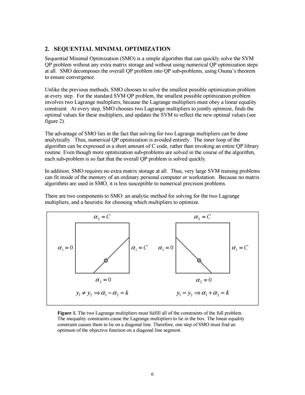
2.SEQUENTIAL MINIMAL OPTIMIZATION Sequential Minimal Optimization(SMO)is a simple algorithm that can quickly solve the SVM QP problem without any extra matrix storage and without using numerical QP optimization steps at all.SMO decomposes the overall QP problem into QP sub-problems,using Osuna's theorem to ensure convergence. Unlike the previous methods,SMO chooses to solve the smallest possible optimization problem at every step.For the standard SVM QP problem,the smallest possible optimization problem involves two Lagrange multipliers,because the Lagrange multipliers must obey a linear equality constraint.At every step,SMO chooses two Lagrange multipliers to jointly optimize,finds the optimal values for these multipliers,and updates the SVM to reflect the new optimal values(see figure 2). The advantage of SMO lies in the fact that solving for two Lagrange multipliers can be done analytically.Thus,numerical QP optimization is avoided entirely.The inner loop of the algorithm can be expressed in a short amount of C code,rather than invoking an entire QP library routine.Even though more optimization sub-problems are solved in the course of the algorithm, each sub-problem is so fast that the overall QP problem is solved quickly. In addition,SMO requires no extra matrix storage at all.Thus,very large SVM training problems can fit inside of the memory of an ordinary personal computer or workstation.Because no matrix algorithms are used in SMO,it is less susceptible to numerical precision problems. There are two components to SMO:an analytic method for solving for the two Lagrange multipliers,and a heuristic for choosing which multipliers to optimize. a,=C a,=C a1=0 a=C 0x1=0 =C 02=0 x2=0 y≠y3→0x1-02=k 片=2→01+0x2=k Figure 1.The two Lagrange multipliers must fulfill all of the constraints of the full problem. The inequality constraints cause the Lagrange multipliers to lie in the box.The linear equality constraint causes them to lie on a diagonal line.Therefore,one step of SMO must find an optimum of the objective function on a diagonal line segment. 66 2. SEQUENTIAL MINIMAL OPTIMIZATION Sequential Minimal Optimization (SMO) is a simple algorithm that can quickly solve the SVM QP problem without any extra matrix storage and without using numerical QP optimization steps at all. SMO decomposes the overall QP problem into QP sub-problems, using Osuna’s theorem to ensure convergence. Unlike the previous methods, SMO chooses to solve the smallest possible optimization problem at every step. For the standard SVM QP problem, the smallest possible optimization problem involves two Lagrange multipliers, because the Lagrange multipliers must obey a linear equality constraint. At every step, SMO chooses two Lagrange multipliers to jointly optimize, finds the optimal values for these multipliers, and updates the SVM to reflect the new optimal values (see figure 2). The advantage of SMO lies in the fact that solving for two Lagrange multipliers can be done analytically. Thus, numerical QP optimization is avoided entirely. The inner loop of the algorithm can be expressed in a short amount of C code, rather than invoking an entire QP library routine. Even though more optimization sub-problems are solved in the course of the algorithm, each sub-problem is so fast that the overall QP problem is solved quickly. In addition, SMO requires no extra matrix storage at all. Thus, very large SVM training problems can fit inside of the memory of an ordinary personal computer or workstation. Because no matrix algorithms are used in SMO, it is less susceptible to numerical precision problems. There are two components to SMO: an analytic method for solving for the two Lagrange multipliers, and a heuristic for choosing which multipliers to optimize. Figure 1. The two Lagrange multipliers must fulfill all of the constraints of the full problem. The inequality constraints cause the Lagrange multipliers to lie in the box. The linear equality constraint causes them to lie on a diagonal line. Therefore, one step of SMO must find an optimum of the objective function on a diagonal line segment. a2 = C a2 = C a2 = 0 a1 = 0 a1 = C yy k 12 12 ¡Æ- = a a a2 = 0 a1 = 0 a1 = C yy k 12 12 =Æ+ = a a