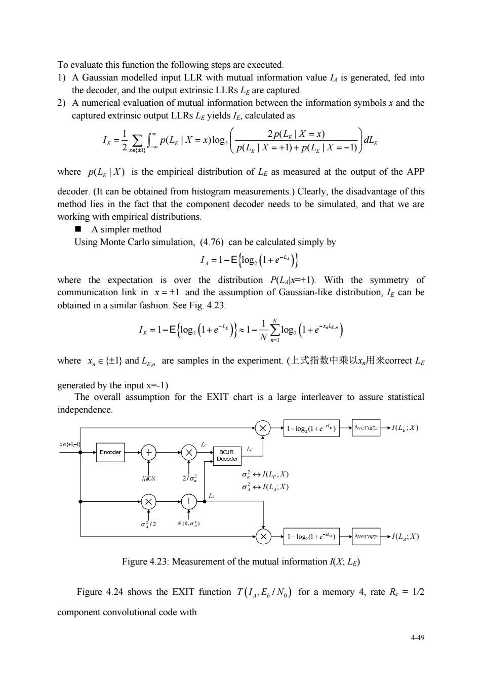
To evaluate this function the following steps are executed. 1)A Gaussian modelled input LLR with mutual information value L is generated,fed into the decoder,and the oupu textrinsic LLRsL are captured 2)A numerical evaluation of mutual information between the information symbolsx and the captured extrinsic output LLRs LE yields I,calculated as =∑plX=log 2p(LelX=x) p(LX=)+p(LX=-DdLe where p(L)is the empirical distribution of Le as measured at the output of the APP decoder.(It can be obtained from histogram measurements.)Clearly,the disadvantage of this method lies in the fact that the component decoder needs to be simulated,and that we are working with empirical distributions Asimpler method Using Monte Carlo simulation,(4.76)can be calculated simply by 14=1-E1og,（1+eb)）} 兰2w and the a ssumption of Ga n-like distribution,can be 11-og (o) where xe{仕l)andL are samples in the experiment.(上式指数中乘以xn用来correct L assumption for the EXIT chart is a large interleaver to assure statistical independence ☒一e,0+e-ee) A o←+IL,X) Lx) 14 X(0.c) 又-1-log,l+e)Averse1亿：X0 Figure 4.23:Measurement of the mutual information I(X;L) Figure 4.24 shows the EXIT function T(E/No)for a memory 4,rate Re 1/2 component convolutional code with 449 4-49 To evaluate this function the following steps are executed. 1) A Gaussian modelled input LLR with mutual information value IA is generated, fed into the decoder, and the output extrinsic LLRs LE are captured. 2) A numerical evaluation of mutual information between the information symbols x and the captured extrinsic output LLRs LE yields IE, calculated as 2 { 1} 1 2( | ) ( | )log 2 ( | 1) ( | 1) E E E E x E E pL X x I p L X x dL pL X pL X                   where ( | ) E p L X is the empirical distribution of LE as measured at the output of the APP decoder. (It can be obtained from histogram measurements.) Clearly, the disadvantage of this method lies in the fact that the component decoder needs to be simulated, and that we are working with empirical distributions.  A simpler method Using Monte Carlo simulation, (4.76) can be calculated simply by 1 log 1  2   LA AI e   E where the expectation is over the distribution P(LA|x=+1). With the symmetry of communication link in x  1 and the assumption of Gaussian-like distribution, IE can be obtained in a similar fashion. See Fig. 4.23.       , 2 2 1 1 1 log 1 1 log 1 E n En N L x L E n Ie e N        E  where , { 1} and n En x   L are samples in the experiment. (上式指数中乘以xn用来correct LE generated by the input x=-1) The overall assumption for the EXIT chart is a large interleaver to assure statistical independence. 2 2/ n 1 log (1 ) 2 E xL e   I(L ; X ) E I(L ; X ) A ( ; ) ( ; ) 2 2 I L X I L X A A n C     1 log (1 ) 2 A xL e   / 2 2  A (0, ) 2 N  A x{1,1} Figure 4.23: Measurement of the mutual information I(X; LE) Figure 4.24 shows the EXIT function TI E N  A b , / 0  for a memory 4, rate Rc = 1/2 component convolutional code with