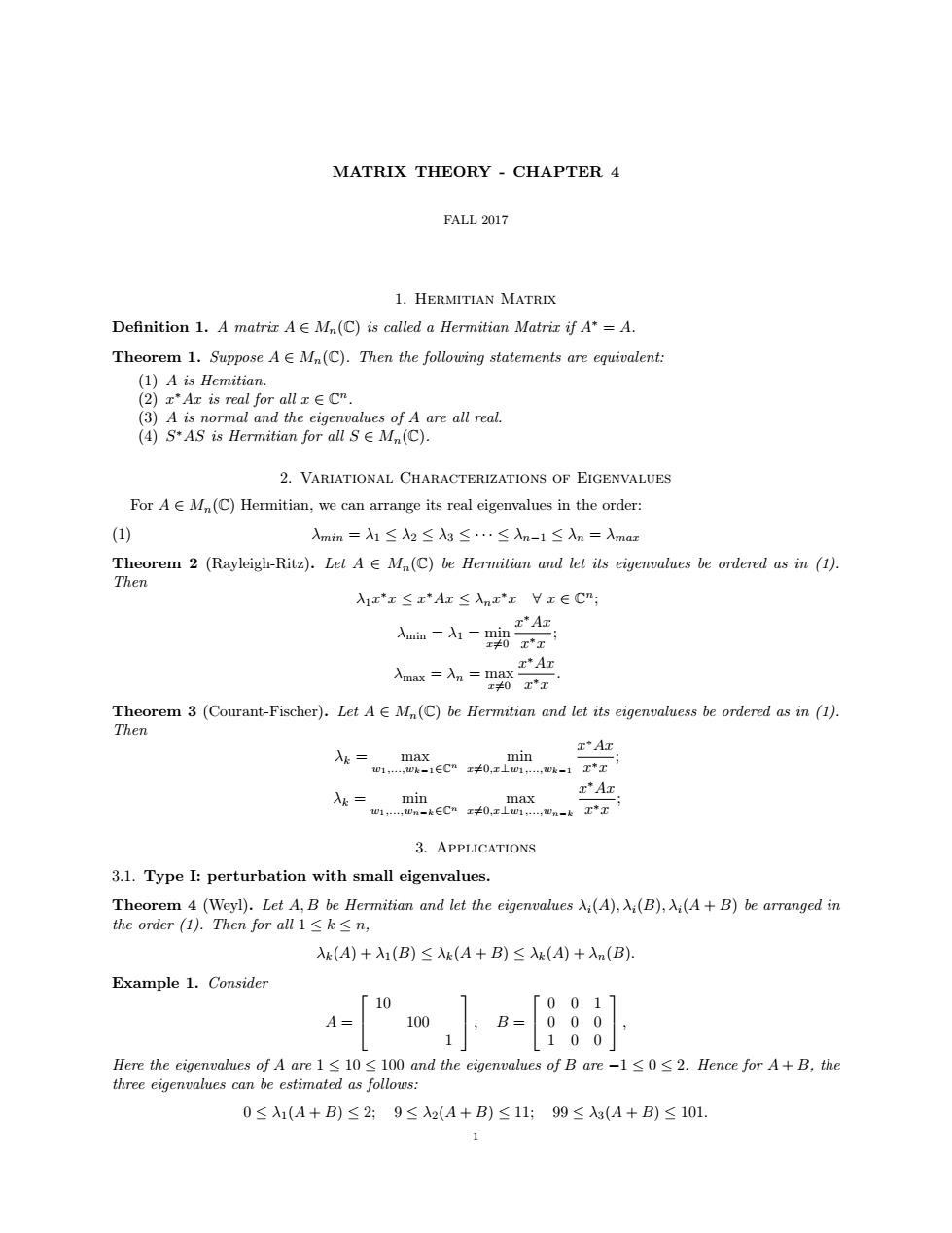
MATRIX THEORY CHAPTER 4 FALL 2017 1.HERMITIAN MATRIX Definition 1.A matrir AE Mn(C)is called a Hermitian Matrir if A"=A. Theorem 1.Suppose AM(C).Then the following statements are equivalent: (3)A is normal and the eigenvalues of A are all real. (4)④S*AS is Hermitian for all S∈Mn(C). 2.VARIATIONAL CHARACTERIZATIONS OF EIGENVALUES For AM(C)Hermitian,we can arrange its real eigenvalues in the order: ) 入mn=1≤h≤3≤…≤入n-l≤n=Amam Theorem 2 (Rayleigh-Ritz).Let AE M(C)be Hermitian and let its eigenvalues be ordered as in (1). Then Axx≤xAr≤nr'xVx∈C ==男碧 Theorem 3 (Courant-Fischer).Let AEM(C)be Hermitian and let its eigenvaluess be ordered as in (1). Then r'Ar 3.APPLICATIONS 3.1.Type I:perturbation with small eigenvalues. Then for Ak(A)+A1(B)≤Xk(A+B)≤X(A)+A(B). Example 1.Consider 10 ,B= 「0011 A= 100 L1. Here the eigenlueso时Aae1≤10≤100 and the eigenvalues of B are-l≤0≤2.Hence for A+B,the three eigenvalues can be estimated as follows: 0≤A(A+B)≤2：9≤A2(A+B)≤11：99≤(4+B)≤101MATRIX THEORY - CHAPTER 4 FALL 2017 1. Hermitian Matrix Definition 1. A matrix A ∈ Mn(C) is called a Hermitian Matrix if A∗ = A. Theorem 1. Suppose A ∈ Mn(C). Then the following statements are equivalent: (1) A is Hemitian. (2) x ∗Ax is real for all x ∈ C n. (3) A is normal and the eigenvalues of A are all real. (4) S ∗AS is Hermitian for all S ∈ Mn(C). 2. Variational Characterizations of Eigenvalues For A ∈ Mn(C) Hermitian, we can arrange its real eigenvalues in the order: (1) λmin = λ1 ≤ λ2 ≤ λ3 ≤ · · · ≤ λn−1 ≤ λn = λmax Theorem 2 (Rayleigh-Ritz). Let A ∈ Mn(C) be Hermitian and let its eigenvalues be ordered as in (1). Then λ1x ∗x ≤ x ∗Ax ≤ λnx ∗x ∀ x ∈ C n ; λmin = λ1 = min x6=0 x ∗Ax x ∗x ; λmax = λn = max x6=0 x ∗Ax x ∗x . Theorem 3 (Courant-Fischer). Let A ∈ Mn(C) be Hermitian and let its eigenvaluess be ordered as in (1). Then λk = max w1,...,wk−1∈Cn min x6=0,x⊥w1,...,wk−1 x ∗Ax x ∗x ; λk = min w1,...,wn−k∈Cn max x6=0,x⊥w1,...,wn−k x ∗Ax x ∗x ; 3. Applications 3.1. Type I: perturbation with small eigenvalues. Theorem 4 (Weyl). Let A, B be Hermitian and let the eigenvalues λi(A), λi(B), λi(A + B) be arranged in the order (1). Then for all 1 ≤ k ≤ n, λk(A) + λ1(B) ≤ λk(A + B) ≤ λk(A) + λn(B). Example 1. Consider A =   10 100 1   , B =   0 0 1 0 0 0 1 0 0   , Here the eigenvalues of A are 1 ≤ 10 ≤ 100 and the eigenvalues of B are −1 ≤ 0 ≤ 2. Hence for A + B, the three eigenvalues can be estimated as follows: 0 ≤ λ1(A + B) ≤ 2; 9 ≤ λ2(A + B) ≤ 11; 99 ≤ λ3(A + B) ≤ 101. 1