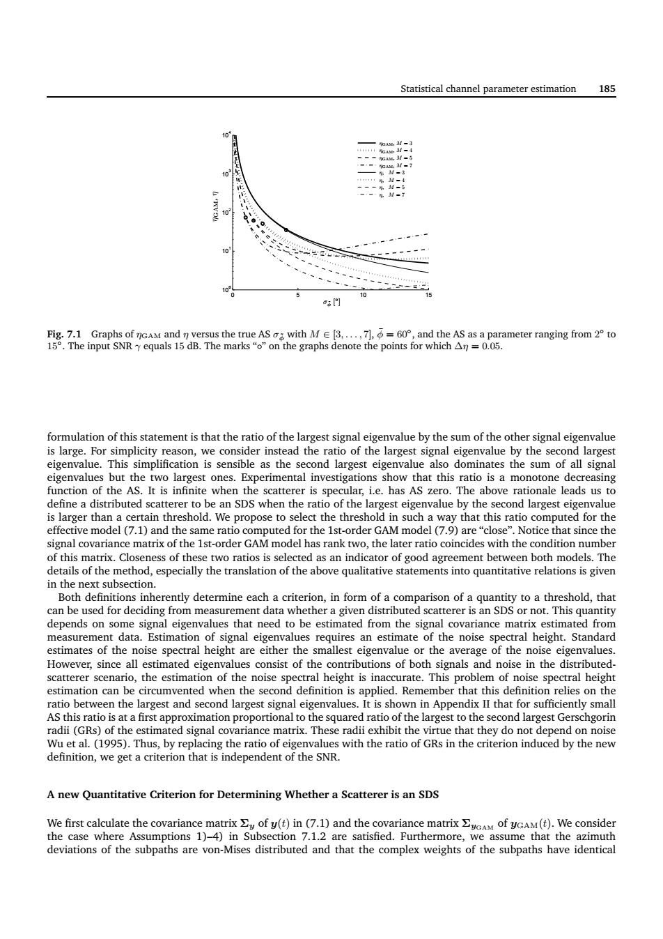
Statistical channel parameter estimation 185 3門 hamrer ranging from2to eigenvalue define a distributed scatterer to be an SDS when the ratio of the la eigenvalue by the second largest signal covariance matrix of the Ist-order GAM model has rank two,the later ratio coincides with the condition number in the next subsection hold,that mal cigenvalues that need to be estimated from the sisal covariance matrix estimated from measurement data.Estimation o ral height.Standard e in the distributed noise spectral heigh AS this ratio is at a first approximation proportional to th aedaiofthelargeotheseondlagetcenchgoin definition,we get a criterion that is independent of the SNR. A new Quantitative Criterion for Determining Whether a Scatterer is an SDS n7.1. Statistical channel parameter estimation 185 0 5 10 15 100 101 102 103 104 ηGAM, M = 3 ηGAM, M = 4 ηGAM, M = 5 ηGAM, M = 7 η, M = 3 η, M = 4 η, M = 5 η, M = 7 σφ˜ [ ◦ ] ηGAM, η Fig. 7.1 Graphs of ηGAM and η versus the true AS σφ˜ with M ∈ [3, . . . , 7], φ¯ = 60◦ , and the AS as a parameter ranging from 2 ◦ to 15◦ . The input SNR γ equals 15 dB. The marks “◦” on the graphs denote the points for which ∆η = 0.05. formulation of this statement is that the ratio of the largest signal eigenvalue by the sum of the other signal eigenvalue is large. For simplicity reason, we consider instead the ratio of the largest signal eigenvalue by the second largest eigenvalue. This simplification is sensible as the second largest eigenvalue also dominates the sum of all signal eigenvalues but the two largest ones. Experimental investigations show that this ratio is a monotone decreasing function of the AS. It is infinite when the scatterer is specular, i.e. has AS zero. The above rationale leads us to define a distributed scatterer to be an SDS when the ratio of the largest eigenvalue by the second largest eigenvalue is larger than a certain threshold. We propose to select the threshold in such a way that this ratio computed for the effective model (7.1) and the same ratio computed for the 1st-order GAM model (7.9) are “close”. Notice that since the signal covariance matrix of the 1st-order GAM model has rank two, the later ratio coincides with the condition number of this matrix. Closeness of these two ratios is selected as an indicator of good agreement between both models. The details of the method, especially the translation of the above qualitative statements into quantitative relations is given in the next subsection. Both definitions inherently determine each a criterion, in form of a comparison of a quantity to a threshold, that can be used for deciding from measurement data whether a given distributed scatterer is an SDS or not. This quantity depends on some signal eigenvalues that need to be estimated from the signal covariance matrix estimated from measurement data. Estimation of signal eigenvalues requires an estimate of the noise spectral height. Standard estimates of the noise spectral height are either the smallest eigenvalue or the average of the noise eigenvalues. However, since all estimated eigenvalues consist of the contributions of both signals and noise in the distributed￾scatterer scenario, the estimation of the noise spectral height is inaccurate. This problem of noise spectral height estimation can be circumvented when the second definition is applied. Remember that this definition relies on the ratio between the largest and second largest signal eigenvalues. It is shown in Appendix II that for sufficiently small AS this ratio is at a first approximation proportional to the squared ratio of the largest to the second largest Gerschgorin radii (GRs) of the estimated signal covariance matrix. These radii exhibit the virtue that they do not depend on noise Wu et al. (1995). Thus, by replacing the ratio of eigenvalues with the ratio of GRs in the criterion induced by the new definition, we get a criterion that is independent of the SNR. A new Quantitative Criterion for Determining Whether a Scatterer is an SDS We first calculate the covariance matrix Σy of y(t) in (7.1) and the covariance matrix ΣyGAM of yGAM(t). We consider the case where Assumptions 1)–4) in Subsection 7.1.2 are satisfied. Furthermore, we assume that the azimuth deviations of the subpaths are von-Mises distributed and that the complex weights of the subpaths have identical