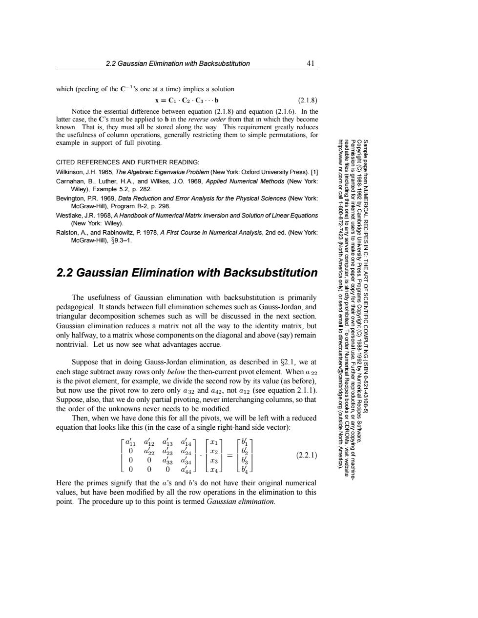
2.2 Gaussian Elimination with Backsubstitution 41 which (peeling of the C-'s one at a time)implies a solution x=C1.C2.C3..b (2.1.8) Notice the essential difference between equation (2.1.8)and equation (2.1.6).In the latter case,the C's must be applied to b in the reverse order from that in which they become known.That is,they must all be stored along the way.This requirement greatly reduces the usefulness of column operations,generally restricting them to simple permutations,for example in support of full pivoting. CITED REFERENCES AND FURTHER READING: Wilkinson,J.H.1965,The Algebraic Eigenvalue Problem (New York:Oxford University Press).[1] Carnahan,B.,Luther,H.A,and Wilkes,J.O.1969.Applied Numerical Methods (New York: Wiley),Example 5.2,p.282. Bevington,P.R.1969,Data Reduction and Error Analysis for the Physical Sciences (New York: McGraw-Hill),Program B-2,p.298. Westlake,J.R.1968,A Handbook of Numerical Matrix Inversion and Solution of Linear Equations (New York:Wiley). Ralston,A.,and Rabinowitz,P.1978,A First Course in Numerica/Analysis,2nd ed.(New York: 巡 McGraw-Hill),89.3-1. 9 令 2.2 Gaussian Elimination with Backsubstitution Press. The usefulness of Gaussian elimination with backsubstitution is primarily Programs pedagogical.It stands between full elimination schemes such as Gauss-Jordan,and triangular decomposition schemes such as will be discussed in the next section. SCIENTIFIC Gaussian elimination reduces a matrix not all the way to the identity matrix,but only halfway,to a matrix whose components on the diagonal and above(say)remain 排 6 nontrivial.Let us now see what advantages accrue. Suppose that in doing Gauss-Jordan elimination,as described in 82.1,we at each stage subtract away rows only below the then-current pivot element.When a 22 is the pivot element,for example,we divide the second row by its value(as before), 10.621 but now use the pivot row to zero only a32 and a42,not a12 (see equation 2.1.1). Numerica Suppose,also,that we do only partial pivoting,never interchanging columns,so that 431 the order of the unknowns never needs to be modified. uction Then,when we have done this for all the pivots,we will be left with a reduced Recipes equation that looks like this(in the case of a single right-hand side vector): (outside a11 a12 a13 a14 T1 North 0 a22 023 T2 (2.2.1) 0 0 33 T3 0 0 44 4」 Here the primes signify that the a's and b's do not have their original numerical values,but have been modified by all the row operations in the elimination to this point.The procedure up to this point is termed Gaussian elimination.2.2 Gaussian Elimination with Backsubstitution 41 Permission is granted for internet users to make one paper copy for their own personal use. Further reproduction, or any copyin Copyright (C) 1988-1992 by Cambridge University Press. Programs Copyright (C) 1988-1992 by Numerical Recipes Software. Sample page from NUMERICAL RECIPES IN C: THE ART OF SCIENTIFIC COMPUTING (ISBN 0-521-43108-5) g of machine￾readable files (including this one) to any server computer, is strictly prohibited. To order Numerical Recipes books or CDROMs, visit website http://www.nr.com or call 1-800-872-7423 (North America only), or send email to directcustserv@cambridge.org (outside North America). which (peeling of the C−1’s one at a time) implies a solution x = C1 · C2 · C3 ··· b (2.1.8) Notice the essential difference between equation (2.1.8) and equation (2.1.6). In the latter case, the C’s must be applied to b in the reverse order from that in which they become known. That is, they must all be stored along the way. This requirement greatly reduces the usefulness of column operations, generally restricting them to simple permutations, for example in support of full pivoting. CITED REFERENCES AND FURTHER READING: Wilkinson, J.H. 1965, The Algebraic Eigenvalue Problem (New York: Oxford University Press). [1] Carnahan, B., Luther, H.A., and Wilkes, J.O. 1969, Applied Numerical Methods (New York: Wiley), Example 5.2, p. 282. Bevington, P.R. 1969, Data Reduction and Error Analysis for the Physical Sciences (New York: McGraw-Hill), Program B-2, p. 298. Westlake, J.R. 1968, A Handbook of Numerical Matrix Inversion and Solution of Linear Equations (New York: Wiley). Ralston, A., and Rabinowitz, P. 1978, A First Course in Numerical Analysis, 2nd ed. (New York: McGraw-Hill), §9.3–1. 2.2 Gaussian Elimination with Backsubstitution The usefulness of Gaussian elimination with backsubstitution is primarily pedagogical. It stands between full elimination schemes such as Gauss-Jordan, and triangular decomposition schemes such as will be discussed in the next section. Gaussian elimination reduces a matrix not all the way to the identity matrix, but only halfway, to a matrix whose components on the diagonal and above (say) remain nontrivial. Let us now see what advantages accrue. Suppose that in doing Gauss-Jordan elimination, as described in §2.1, we at each stage subtract away rows only below the then-current pivot element. When a 22 is the pivot element, for example, we divide the second row by its value (as before), but now use the pivot row to zero only a32 and a42, not a12 (see equation 2.1.1). Suppose, also, that we do only partial pivoting, never interchanging columns, so that the order of the unknowns never needs to be modified. Then, when we have done this for all the pivots, we will be left with a reduced equation that looks like this (in the case of a single right-hand side vector):    a
11 a
12 a
13 a
14 0 a
22 a
23 a
24 0 0 a
33 a
34 000 a
44    ·    x1 x2 x3 x4    =    b
1 b
2 b
3 b
4    (2.2.1) Here the primes signify that the a’s and b’s do not have their original numerical values, but have been modified by all the row operations in the elimination to this point. The procedure up to this point is termed Gaussian elimination