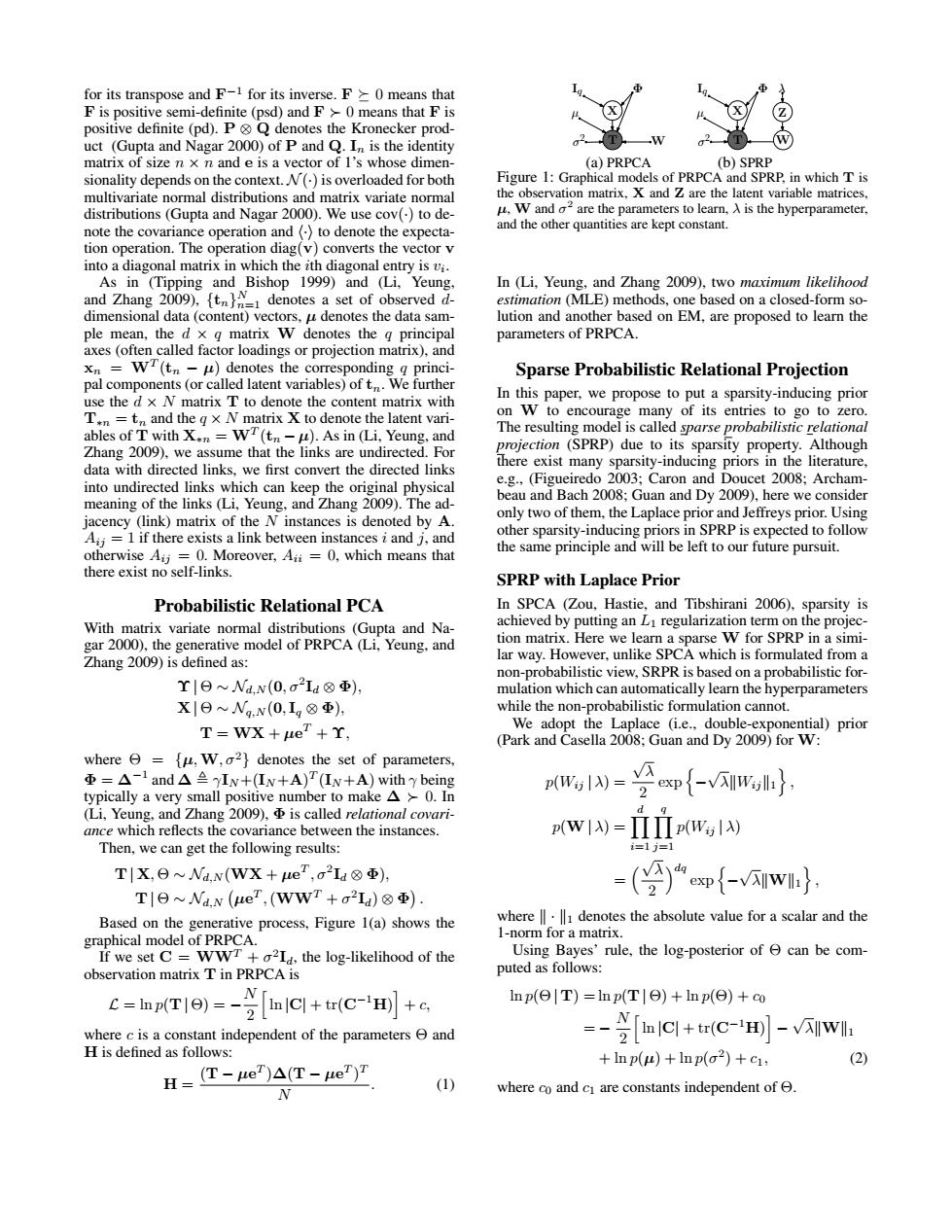
for its transpose and F-1 for its inverse.F0 means that F is positive semi-definite(psd)and F0 means that F is positive definite (pd).PQ denotes the Kronecker prod- uct (Gupta and Nagar 2000)of P and Q.In is the identity matrix of size n x n and e is a vector of I's whose dimen- (a)PRPCA (b)SPRP sionality depends on the context.N()is overloaded for both Figure 1:Graphical models of PRPCA and SPRP,in which T is multivariate normal distributions and matrix variate normal the observation matrix,X and Z are the latent variable matrices, distributions(Gupta and Nagar 2000).We use cov()to de- μ，W and a2 are the parameters to learn,入is the hyperparameter, note the covariance operation and()to denote the expecta- and the other quantities are kept constant. tion operation.The operation diag(v)converts the vector v into a diagonal matrix in which the ith diagonal entry is vi. As in (Tipping and Bishop 1999)and (Li,Yeung, In (Li,Yeung,and Zhang 2009),two maximum likelihood and Zhang 2009).denotes a set of observed d- estimation (MLE)methods,one based on a closed-form so- dimensional data (content)vectors,u denotes the data sam- lution and another based on EM,are proposed to learn the ple mean,the d x q matrix W denotes the g principal parameters of PRPCA. axes (often called factor loadings or projection matrix),and xn=WT(tn-u)denotes the corresponding g princi- Sparse Probabilistic Relational Projection pal components (or called latent variables)of t.We further use the d x N matrix T to denote the content matrix with In this paper,we propose to put a sparsity-inducing prior T=tn and the g x N matrix X to denote the latent vari- on W to encourage many of its entries to go to zero. ables of T with X.n=WT(tn -u).As in (Li,Yeung,and The resulting model is called sparse probabilistic relational Zhang 2009),we assume that the links are undirected.For projection(SPRP)due to its sparsity property.Although data with directed links,we first convert the directed links there exist many sparsity-inducing priors in the literature, into undirected links which can keep the original physical e.g.,(Figueiredo 2003;Caron and Doucet 2008;Archam- meaning of the links (Li,Yeung,and Zhang 2009).The ad- beau and Bach 2008;Guan and Dy 2009),here we consider jacency (link)matrix of the N instances is denoted by A. only two of them,the Laplace prior and Jeffreys prior.Using Aij =1 if there exists a link between instances i and j,and other sparsity-inducing priors in SPRP is expected to follow otherwise Aij=0.Moreover,A =0,which means that the same principle and will be left to our future pursuit. there exist no self-links. SPRP with Laplace Prior Probabilistic Relational PCA In SPCA (Zou,Hastie,and Tibshirani 2006),sparsity is With matrix variate normal distributions (Gupta and Na- achieved by putting an LI regularization term on the projec- gar 2000),the generative model of PRPCA (Li,Yeung.and tion matrix.Here we learn a sparse W for SPRP in a simi- Zhang 2009)is defined as: lar way.However,unlike SPCA which is formulated from a non-probabilistic view,SRPR is based on a probabilistic for- Y1日~Na,N(0,oIa⑧Φ) mulation which can automatically learn the hyperparameters X|日~Ng,N(0,Ig⑧Φ) while the non-probabilistic formulation cannot. T=WX+ueT+T. We adopt the Laplace (i.e.,double-exponential)prior (Park and Casella 2008;Guan and Dy 2009)for W: where e=fu,W,o2}denotes the set of parameters, ④=△-1and△≌Iw+(Iw+A)T(Iw+A)with being typically a very small positive number to make A 0.In )pf-v} (Li,Yeung,and Zhang 2009).is called relational covari- ance which reflects the covariance between the instances. (wI)=ΠΠ(W1) Then,we can get the following results: T|X,日~Na,v(WX+ueT,a2L48Φ) -()"oxpf-/wi}. T|日~Na,N(ueT,(WWr+aIa)⑧Φ). Based on the generative process,Figure 1(a)shows the where lll denotes the absolute value for a scalar and the graphical model of PRPCA. I-norm for a matrix. If we set C WWT+o2Id,the log-likelihood of the Using Bayes'rule,the log-posterior of e can be com- observation matrix T in PRPCA is puted as follows: c=aTIe)=-yac+c-到+ lnp(Θ|T)=lnp(TlΘ)+lnp(Θ)+co where c is a constant independent of the parameters e and =-Yac+(c-到-vw: H is defined as follows: +Inp(u)+Inp(o2)+c1, (2) H=T-ue)△(T-ue)Y (1) where co and cI are constants independent offor its transpose and F −1 for its inverse. F  0 means that F is positive semi-definite (psd) and F  0 means that F is positive definite (pd). P ⊗ Q denotes the Kronecker prod￾uct (Gupta and Nagar 2000) of P and Q. In is the identity matrix of size n × n and e is a vector of 1’s whose dimen￾sionality depends on the context. N (·) is overloaded for both multivariate normal distributions and matrix variate normal distributions (Gupta and Nagar 2000). We use cov(·) to de￾note the covariance operation and h·i to denote the expecta￾tion operation. The operation diag(v) converts the vector v into a diagonal matrix in which the ith diagonal entry is vi . As in (Tipping and Bishop 1999) and (Li, Yeung, and Zhang 2009), {tn} N n=1 denotes a set of observed d￾dimensional data (content) vectors, µ denotes the data sam￾ple mean, the d × q matrix W denotes the q principal axes (often called factor loadings or projection matrix), and xn = WT (tn − µ) denotes the corresponding q princi￾pal components (or called latent variables) of tn. We further use the d × N matrix T to denote the content matrix with T∗n = tn and the q × N matrix X to denote the latent vari￾ables of T with X∗n = WT (tn −µ). As in (Li, Yeung, and Zhang 2009), we assume that the links are undirected. For data with directed links, we first convert the directed links into undirected links which can keep the original physical meaning of the links (Li, Yeung, and Zhang 2009). The ad￾jacency (link) matrix of the N instances is denoted by A. Aij = 1 if there exists a link between instances i and j, and otherwise Aij = 0. Moreover, Aii = 0, which means that there exist no self-links. Probabilistic Relational PCA With matrix variate normal distributions (Gupta and Na￾gar 2000), the generative model of PRPCA (Li, Yeung, and Zhang 2009) is defined as: Υ | Θ ∼ Nd,N (0, σ2 Id ⊗ Φ), X | Θ ∼ Nq,N (0, Iq ⊗ Φ), T = WX + µe T + Υ, where Θ = {µ,W, σ2} denotes the set of parameters, Φ = ∆−1 and ∆ , γIN +(IN +A) T (IN +A) with γ being typically a very small positive number to make ∆  0. In (Li, Yeung, and Zhang 2009), Φ is called relational covari￾ance which reflects the covariance between the instances. Then, we can get the following results: T | X, Θ ∼ Nd,N (WX + µe T , σ2 Id ⊗ Φ), T | Θ ∼ Nd,N ￾ µe T ,(WWT + σ 2 Id) ⊗ Φ
. Based on the generative process, Figure 1(a) shows the graphical model of PRPCA. If we set C = WWT + σ 2 Id, the log-likelihood of the observation matrix T in PRPCA is L = ln p(T | Θ) = − N 2 h ln |C| + tr(C−1H) i + c, where c is a constant independent of the parameters Θ and H is defined as follows: H = (T − µe T )∆(T − µe T ) T N . (1) T X Iq σ 2 W µ Φ T X Iq σ 2 W µ Φ Z λ (a) PRPCA (b) SPRP Figure 1: Graphical models of PRPCA and SPRP, in which T is the observation matrix, X and Z are the latent variable matrices, µ, W and σ 2 are the parameters to learn, λ is the hyperparameter, and the other quantities are kept constant. In (Li, Yeung, and Zhang 2009), two maximum likelihood estimation (MLE) methods, one based on a closed-form so￾lution and another based on EM, are proposed to learn the parameters of PRPCA. Sparse Probabilistic Relational Projection In this paper, we propose to put a sparsity-inducing prior on W to encourage many of its entries to go to zero. The resulting model is called sparse probabilistic relational projection (SPRP) due to its sparsity property. Although there exist many sparsity-inducing priors in the literature, e.g., (Figueiredo 2003; Caron and Doucet 2008; Archam￾beau and Bach 2008; Guan and Dy 2009), here we consider only two of them, the Laplace prior and Jeffreys prior. Using other sparsity-inducing priors in SPRP is expected to follow the same principle and will be left to our future pursuit. SPRP with Laplace Prior In SPCA (Zou, Hastie, and Tibshirani 2006), sparsity is achieved by putting an L1 regularization term on the projec￾tion matrix. Here we learn a sparse W for SPRP in a simi￾lar way. However, unlike SPCA which is formulated from a non-probabilistic view, SRPR is based on a probabilistic for￾mulation which can automatically learn the hyperparameters while the non-probabilistic formulation cannot. We adopt the Laplace (i.e., double-exponential) prior (Park and Casella 2008; Guan and Dy 2009) for W: p(Wij | λ) = √ λ 2 exp n − √ λkWijk1 o , p(W| λ) = Y d i=1 Yq j=1 p(Wij | λ) =  √ λ 2 dq exp n − √ λkWk1 o , where k · k1 denotes the absolute value for a scalar and the 1-norm for a matrix. Using Bayes’ rule, the log-posterior of Θ can be com￾puted as follows: ln p(Θ | T) = ln p(T | Θ) + ln p(Θ) + c0 = − N 2 h ln |C| + tr(C−1H) i − √ λkWk1 + ln p(µ) + ln p(σ 2 ) + c1, (2) where c0 and c1 are constants independent of Θ