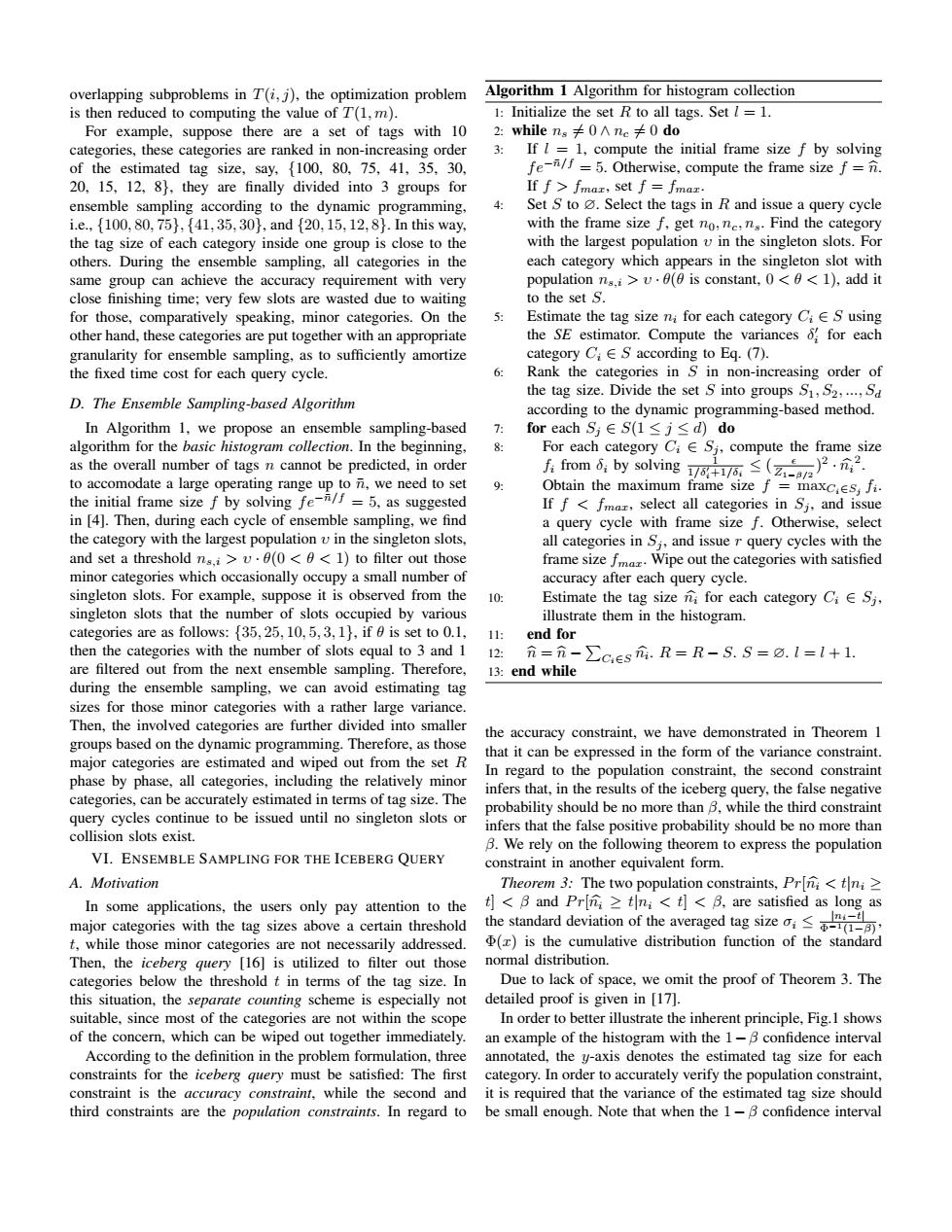
overlapping subproblems in T(i,j),the optimization problem Algorithm 1 Algorithm for histogram collection is then reduced to computing the value of T(1,m). 1:Initialize the set R to all tags.Set l=1. For example,suppose there are a set of tags with 10 2:while ns≠0Ane≠0do categories,these categories are ranked in non-increasing order 3: If I=1,compute the initial frame size f by solving of the estimated tag size,say,{100,80,75,41,35,30, fe-/=5.Otherwise,compute the frame size f=n. 20,15,12,8,they are finally divided into 3 groups for If f>fmaz,set f=fmaz. ensemble sampling according to the dynamic programming, 4 Set S to Select the tags in R and issue a query cycle i.e.,{100,80,75},{41,35,30,and{20,15,12,8.In this way,. with the frame size f,get no,ne,n Find the category the tag size of each category inside one group is close to the with the largest population v in the singleton slots.For others.During the ensemble sampling,all categories in the each category which appears in the singleton slot with same group can achieve the accuracy requirement with very population ns.i>v.(is constant,0<<1),add it close finishing time;very few slots are wasted due to waiting to the set S. for those,comparatively speaking,minor categories.On the 5: Estimate the tag size ni for each category CiE S using other hand,these categories are put together with an appropriate the SE estimator.Compute the variances for each granularity for ensemble sampling,as to sufficiently amortize category C;E S according to Eq.(7). the fixed time cost for each query cycle. 6: Rank the categories in S in non-increasing order of the tag size.Divide the set S into groups S1,S2,...,Sa D.The Ensemble Sampling-based Algorithm according to the dynamic programming-based method. In Algorithm 1,we propose an ensemble sampling-based 7: for each S∈S(1≤j≤d)do algorithm for the basic histogram collection.In the beginning, 8: For each category CiE Sj,compute the frame size as the overall number of tags n cannot be predicted,in order f:from 6,by solving7a47石≤(zae2.i2. to accomodate a large operating range up to n,we need to set 9: Obtain the maximum frame size f maxces,fi. the initial frame size f by solving fe/=5,as suggested If f<fmar,select all categories in Sj,and issue in [4].Then,during each cycle of ensemble sampling,we find a query cycle with frame size f.Otherwise,select the category with the largest population v in the singleton slots, all categories in Si,and issue r query cycles with the and set a threshold ns.i>v.(0<<1)to filter out those frame size fma Wipe out the categories with satisfied minor categories which occasionally occupy a small number of accuracy after each query cycle. singleton slots.For example,suppose it is observed from the 10: Estimate the tag size n for each category CiE Sj, singleton slots that the number of slots occupied by various illustrate them in the histogram. categories are as follows:{35,25,10,5,3,1),if 0 is set to 0.1, 11: end for then the categories with the number of slots equal to 3 and 1 12: n=元-∑ces元.R=R-S.S=a.l=l+1. are filtered out from the next ensemble sampling.Therefore, 13:end while during the ensemble sampling,we can avoid estimating tag sizes for those minor categories with a rather large variance. Then,the involved categories are further divided into smaller the accuracy constraint,we have demonstrated in Theorem 1 groups based on the dynamic programming.Therefore,as those that it can be expressed in the form of the variance constraint. major categories are estimated and wiped out from the set R phase by phase,all categories,including the relatively minor In regard to the population constraint,the second constraint infers that,in the results of the iceberg query,the false negative categories,can be accurately estimated in terms of tag size.The query cycles continue to be issued until no singleton slots or probability should be no more than B,while the third constraint infers that the false positive probability should be no more than collision slots exist. B.We rely on the following theorem to express the population VI.ENSEMBLE SAMPLING FOR THE ICEBERG OUERY constraint in another equivalent form. A.Motivation Theorem 3:The two population constraints,Pr[ni<tni> In some applications,the users only pay attention to the t]<B and Pr[i>tni<t]<B.are satisfied as long as the standard deviation of the averaged tag size Ini-tl major categories with the tag sizes above a certain threshold t,while those minor categories are not necessarily addressed. (z)is the cumulative distribution function of the standard Then,the iceberg query [16]is utilized to filter out those normal distribution. categories below the threshold t in terms of the tag size.In Due to lack of space,we omit the proof of Theorem 3.The this situation,the separate counting scheme is especially not detailed proof is given in [17]. suitable,since most of the categories are not within the scope In order to better illustrate the inherent principle,Fig.I shows of the concern,which can be wiped out together immediately.an example of the histogram with the 1-B confidence interval According to the definition in the problem formulation,three annotated,the y-axis denotes the estimated tag size for each constraints for the iceberg query must be satisfied:The first category.In order to accurately verify the population constraint, constraint is the accuracy constraint,while the second and it is required that the variance of the estimated tag size should third constraints are the population constraints.In regard to be small enough.Note that when the 1-B confidence intervaloverlapping subproblems in 𝑇(𝑖, 𝑗), the optimization problem is then reduced to computing the value of 𝑇(1, 𝑚). For example, suppose there are a set of tags with 10 categories, these categories are ranked in non-increasing order of the estimated tag size, say, {100, 80, 75, 41, 35, 30, 20, 15, 12, 8}, they are finally divided into 3 groups for ensemble sampling according to the dynamic programming, i.e., {100, 80, 75}, {41, 35, 30}, and {20, 15, 12, 8}. In this way, the tag size of each category inside one group is close to the others. During the ensemble sampling, all categories in the same group can achieve the accuracy requirement with very close finishing time; very few slots are wasted due to waiting for those, comparatively speaking, minor categories. On the other hand, these categories are put together with an appropriate granularity for ensemble sampling, as to sufficiently amortize the fixed time cost for each query cycle. D. The Ensemble Sampling-based Algorithm In Algorithm 1, we propose an ensemble sampling-based algorithm for the basic histogram collection. In the beginning, as the overall number of tags 𝑛 cannot be predicted, in order to accomodate a large operating range up to 𝑛¯, we need to set the initial frame size 𝑓 by solving 𝑓𝑒−𝑛/𝑓 ¯ = 5, as suggested in [4]. Then, during each cycle of ensemble sampling, we find the category with the largest population 𝜐 in the singleton slots, and set a threshold 𝑛𝑠,𝑖 > 𝜐 ⋅ 𝜃(0 <𝜃< 1) to filter out those minor categories which occasionally occupy a small number of singleton slots. For example, suppose it is observed from the singleton slots that the number of slots occupied by various categories are as follows: {35, 25, 10, 5, 3, 1}, if 𝜃 is set to 0.1, then the categories with the number of slots equal to 3 and 1 are filtered out from the next ensemble sampling. Therefore, during the ensemble sampling, we can avoid estimating tag sizes for those minor categories with a rather large variance. Then, the involved categories are further divided into smaller groups based on the dynamic programming. Therefore, as those major categories are estimated and wiped out from the set 𝑅 phase by phase, all categories, including the relatively minor categories, can be accurately estimated in terms of tag size. The query cycles continue to be issued until no singleton slots or collision slots exist. VI. ENSEMBLE SAMPLING FOR THE ICEBERG QUERY A. Motivation In some applications, the users only pay attention to the major categories with the tag sizes above a certain threshold 𝑡, while those minor categories are not necessarily addressed. Then, the iceberg query [16] is utilized to filter out those categories below the threshold 𝑡 in terms of the tag size. In this situation, the separate counting scheme is especially not suitable, since most of the categories are not within the scope of the concern, which can be wiped out together immediately. According to the definition in the problem formulation, three constraints for the iceberg query must be satisfied: The first constraint is the accuracy constraint, while the second and third constraints are the population constraints. In regard to Algorithm 1 Algorithm for histogram collection 1: Initialize the set 𝑅 to all tags. Set 𝑙 = 1. 2: while 𝑛𝑠 ∕= 0 ∧ 𝑛𝑐 ∕= 0 do 3: If 𝑙 = 1, compute the initial frame size 𝑓 by solving 𝑓𝑒−𝑛/𝑓 ¯ = 5. Otherwise, compute the frame size 𝑓 = 𝑛ˆ. If 𝑓>𝑓𝑚𝑎𝑥, set 𝑓 = 𝑓𝑚𝑎𝑥. 4: Set 𝑆 to ∅. Select the tags in 𝑅 and issue a query cycle with the frame size 𝑓, get 𝑛0, 𝑛𝑐, 𝑛𝑠. Find the category with the largest population 𝜐 in the singleton slots. For each category which appears in the singleton slot with population 𝑛𝑠,𝑖 > 𝜐 ⋅ 𝜃(𝜃 is constant, 0 <𝜃< 1), add it to the set 𝑆. 5: Estimate the tag size 𝑛𝑖 for each category 𝐶𝑖 ∈ 𝑆 using the SE estimator. Compute the variances 𝛿′ 𝑖 for each category 𝐶𝑖 ∈ 𝑆 according to Eq. (7). 6: Rank the categories in 𝑆 in non-increasing order of the tag size. Divide the set 𝑆 into groups 𝑆1, 𝑆2, ..., 𝑆𝑑 according to the dynamic programming-based method. 7: for each 𝑆𝑗 ∈ 𝑆(1 ≤ 𝑗 ≤ 𝑑) do 8: For each category 𝐶𝑖 ∈ 𝑆𝑗 , compute the frame size 𝑓𝑖 from 𝛿𝑖 by solving 1 1/𝛿′ 𝑖+1/𝛿𝑖 ≤ ( 𝜖 𝑍1−𝛽/2 )2 ⋅ 𝑛ˆ𝑖 2 . 9: Obtain the maximum frame size 𝑓 = max𝐶𝑖∈𝑆𝑗 𝑓𝑖. If 𝑓<𝑓𝑚𝑎𝑥, select all categories in 𝑆𝑗 , and issue a query cycle with frame size 𝑓. Otherwise, select all categories in 𝑆𝑗 , and issue 𝑟 query cycles with the frame size 𝑓𝑚𝑎𝑥. Wipe out the categories with satisfied accuracy after each query cycle. 10: Estimate the tag size 𝑛ˆ𝑖 for each category 𝐶𝑖 ∈ 𝑆𝑗 , illustrate them in the histogram. 11: end for 12: 𝑛ˆ = 𝑛ˆ − ∑ 𝐶𝑖∈𝑆 𝑛ˆ𝑖. 𝑅 = 𝑅 − 𝑆. 𝑆 = ∅. 𝑙 = 𝑙 + 1. 13: end while the accuracy constraint, we have demonstrated in Theorem 1 that it can be expressed in the form of the variance constraint. In regard to the population constraint, the second constraint infers that, in the results of the iceberg query, the false negative probability should be no more than 𝛽, while the third constraint infers that the false positive probability should be no more than 𝛽. We rely on the following theorem to express the population constraint in another equivalent form. Theorem 3: The two population constraints, 𝑃 𝑟[𝑛ˆ𝑖 < 𝑡∣𝑛𝑖 ≥ 𝑡] < 𝛽 and 𝑃 𝑟[𝑛ˆ𝑖 ≥ 𝑡∣𝑛𝑖 < 𝑡] < 𝛽, are satisfied as long as the standard deviation of the averaged tag size 𝜎𝑖 ≤ ∣𝑛𝑖−𝑡∣ Φ−1(1−𝛽) , Φ(𝑥) is the cumulative distribution function of the standard normal distribution. Due to lack of space, we omit the proof of Theorem 3. The detailed proof is given in [17]. In order to better illustrate the inherent principle, Fig.1 shows an example of the histogram with the 1−𝛽 confidence interval annotated, the 𝑦-axis denotes the estimated tag size for each category. In order to accurately verify the population constraint, it is required that the variance of the estimated tag size should be small enough. Note that when the 1 − 𝛽 confidence interval