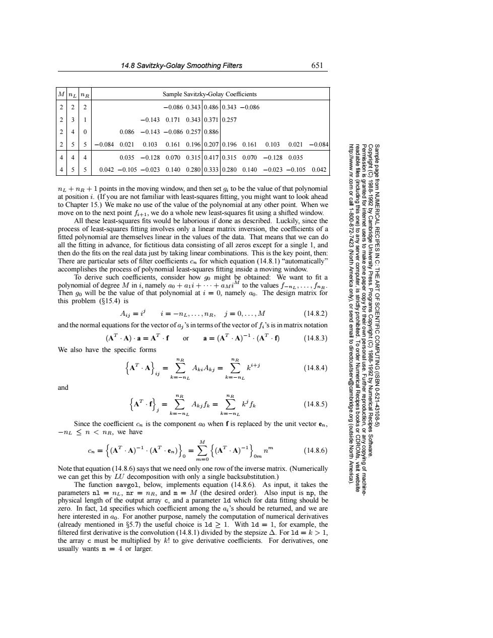
14.8 Savitzky-Golay Smoothing Filters 651 nL nR Sample Savitzky-Golay Coefficients -0.0860.3430.4860.343-0.086 -0.1430.1710.3430.3710.257 2 0 0.086-0.143-0.0860.2570.886 2 -0.0840.0210.1030.1610.1960.2070.1960.1610.1030.021 -0.084 0.035-0.1280.0700.3150.4170.3150.070-0.1280.035 5 0.042-0.105-0.0230.1400.2800.3330.2800.140-0.023-0.1050.042 nL+nR+1 points in the moving window,and then set gi to be the value of that polynomial at position i.(If you are not familiar with least-squares fitting,you might want to look ahead to Chapter 15.)We make no use of the value of the polynomial at any other point.When we nted for move on to the next point f+,we do a whole new least-squares fit using a shifted window. All these least-squares fits would be laborious if done as described.Luckily,since the process of least-squares fitting involves only a linear matrix inversion,the coefficients of a fitted polynomial are themselves linear in the values of the data.That means that we can do all the fitting in advance,for fictitious data consisting of all zeros except for a single 1,and then do the fits on the real data just by taking linear combinations.This is the key point,then: 高A 令 There are particular sets of filter coefficients cn for which equation (14.8.1)"automatically" accomplishes the process of polynomial least-squares fitting inside a moving window. Toderive such cs consider how might obtained:We want tofit a polynomial of degree M in i,namely ao+ai+..+ai" to the values f.-nL,··,JnR Press. Then go will be the value of that polynomial at i 0,namely ao.The design matrix for this problem (815.4)is Programs 9 Aij=ii=-nL;...:nR:j=0,...:M (14.8.2) and the normal equations for the vector of a;'s in terms of the vector of fi's is in matrix notation (AT.A).a=AT.f or a=(AT.A)-1.(AT.f) (14.8.3) 6 We also have the specific forms AA= (14.8.4) k=一nL k三一卫 and {ar.,=定h=2 (14.8.5) Numerical -43126 Since the coefficient c is the component ao when f is replaced by the unit vector en, -n≤n<nr,we have c={aA1.。=∑{a}n (14.8.6) North Software. Note that equation(14.8.6)says that we need only one row of the inverse matrix.(Numerically we can get this by LU decomposition with only a single backsubstitution.) The function savgol,below,implements equation(14.8.6).As input,it takes the parameters nl =nL,nr =nR,and mM(the desired order).Also input is np,the physical length of the output array c,and a parameter ld which for data fitting should be zero.In fact,1d specifies which coefficient among the ai's should be returned,and we are here interested in ao.For another purpose,namely the computation of numerical derivatives (already mentioned in $5.7)the useful choice is ld 1.With ld 1,for example,the filtered first derivative is the convolution (14.8.1)divided by the stepsize A.For ld=>1, the array c must be multiplied by k!to give derivative coefficients.For derivatives,one usually wants m 4 or larger.14.8 Savitzky-Golay Smoothing Filters 651 Permission is granted for internet users to make one paper copy for their own personal use. Further reproduction, or any copyin Copyright (C) 1988-1992 by Cambridge University Press. Programs Copyright (C) 1988-1992 by Numerical Recipes Software. Sample page from NUMERICAL RECIPES IN C: THE ART OF SCIENTIFIC COMPUTING (ISBN 0-521-43108-5) g of machine￾readable files (including this one) to any server computer, is strictly prohibited. To order Numerical Recipes books or CDROMs, visit website http://www.nr.com or call 1-800-872-7423 (North America only), or send email to directcustserv@cambridge.org (outside North America). M nL nR Sample Savitzky-Golay Coefficients 2 2 2 −0.086 0.343 0.486 0.343 −0.086 2 3 1 −0.143 0.171 0.343 0.371 0.257 2 4 0 0.086 −0.143 −0.086 0.257 0.886 2 5 5 −0.084 0.021 0.103 0.161 0.196 0.207 0.196 0.161 0.103 0.021 −0.084 4 4 4 0.035 −0.128 0.070 0.315 0.417 0.315 0.070 −0.128 0.035 4 5 5 0.042 −0.105 −0.023 0.140 0.280 0.333 0.280 0.140 −0.023 −0.105 0.042 nL + nR + 1 points in the moving window, and then set gi to be the value of that polynomial at position i. (If you are not familiar with least-squares fitting, you might want to look ahead to Chapter 15.) We make no use of the value of the polynomial at any other point. When we move on to the next point fi+1, we do a whole new least-squares fit using a shifted window. All these least-squares fits would be laborious if done as described. Luckily, since the process of least-squares fitting involves only a linear matrix inversion, the coefficients of a fitted polynomial are themselves linear in the values of the data. That means that we can do all the fitting in advance, for fictitious data consisting of all zeros except for a single 1, and then do the fits on the real data just by taking linear combinations. This is the key point, then: There are particular sets of filter coefficients cn for which equation (14.8.1) “automatically” accomplishes the process of polynomial least-squares fitting inside a moving window. To derive such coefficients, consider how g0 might be obtained: We want to fit a polynomial of degree M in i, namely a0 + a1i + ··· + aMi M to the values f−nL ,...,fnR . Then g0 will be the value of that polynomial at i = 0, namely a0. The design matrix for this problem (§15.4) is Aij = i j i = −nL,...,nR, j = 0,...,M (14.8.2) and the normal equations for the vector of aj ’s in terms of the vector of fi’s is in matrix notation (AT · A) · a = AT · f or a = (AT · A) −1 · (AT · f) (14.8.3) We also have the specific forms AT · A ij =
nR k=−nL AkiAkj =
nR k=−nL ki+j (14.8.4) and AT · f j =
nR k=−nL Akj fk =
nR k=−nL kj fk (14.8.5) Since the coefficient cn is the component a0 when f is replaced by the unit vector en, −nL ≤ n<nR, we have cn = (AT · A) −1 · (AT · en) 0 =
M m=0 (AT · A) −1 0m nm (14.8.6) Note that equation (14.8.6) says that we need only one row of the inverse matrix. (Numerically we can get this by LU decomposition with only a single backsubstitution.) The function savgol, below, implements equation (14.8.6). As input, it takes the parameters nl = nL, nr = nR, and m = M (the desired order). Also input is np, the physical length of the output array c, and a parameter ld which for data fitting should be zero. In fact, ld specifies which coefficient among the ai’s should be returned, and we are here interested in a0. For another purpose, namely the computation of numerical derivatives (already mentioned in §5.7) the useful choice is ld ≥ 1. With ld = 1, for example, the filtered first derivative is the convolution (14.8.1) divided by the stepsize ∆. For ld = k > 1, the array c must be multiplied by k! to give derivative coefficients. For derivatives, one usually wants m = 4 or larger.