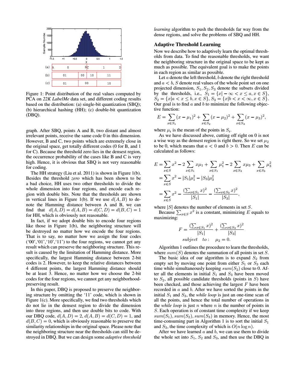
2000 learning algorithm to push the thresholds far way from the 1500 dense regions,and solve the problems of SBQ and HH. Adaptive Threshold Learning Now we describe how to adaptively learn the optimal thresh- olds from data.To find the reasonable thresholds.we want the neighboring structure in the original space to be kept as (a) Bc much as possible.The equivalent goal is to make the points in each region as similar as possible. (b) 00 10 Let a denote the left threshold,b denote the right threshold d 01 00 10 and a <b,S denote real values of the whole point set on one projected dimension,S1,S2,S3 denote the subsets divided Figure 1:Point distribution of the real values computed by by the thresholds,.i.e,S={zl-o<x≤a,x∈S}, PCA on 22K LabelMe data set,and different coding results S2={xla<x≤b,x∈S},S3={xlb<x<o,x∈S}. based on the distribution:(a)single-bit quantization(SBQ); Our goal is to find a and b to minimize the following objec- (b)hierarchical hashing (HH);(c)double-bit quantization tive function: (DBQ). E=∑(x-4)2+∑e-2)2+∑（红-g)2 x∈Sg graph.After SBQ,points A and B,two distant and almost where i is the mean of the points in Si. irrelevant points,receive the same code 0 in this dimension. As we have discussed above,cutting off right on 0 is not However,B and C,two points which are extremely close in a wise way as the densest region is right there.So we set 2 the original space,get totally different codes(0 for B,and 1 to be 0,which means that a <0 and b >0.Then E can be for C).Because the threshold zero lies in the densest region, calculated as follows: the occurrence probability of the cases like B and C is very high.Hence,it is obvious that SBQ is not very reasonable for coding. E=∑2-2∑w+∑-2∑+∑片 IES x∈S1 r∈S1 x∈S3 IESa The HH strategy (Liu et al.2011)is shown in Figure 1(b). Besides the threshold zero which has been shown to be = ∑x2-lSl-lS3lg a bad choice.HH uses two other thresholds to divide the x∈S whole dimension into four regions,and encode each re- gion with double bits.Note that the thresholds are shown =∑x2- (②xs,2_(zs2 in vertical lines in Figure 1(b).If we use d(A,B)to de- xS ISl ISal note the Hamming distance between A and B,we can where S denotes the number of elements in set S. find that d(A.D)=d(A.B)=d(C.D)=d(B.C)=1 for HH,which is obviously not reasonable. Because res2 is a constant,minimizing E equals to maximizing: In fact,if we adopt double bits to encode four regions like those in Figure 1(b),the neighboring structure will be destroyed no matter how we encode the four regions F= (∑zes2(∑es2 S IS3l That is to say,no matter how we assign the four codes (00','01','10','11')to the four regions,we cannot get any subject to:2=0. result which can preserve the neighboring structure.This re- Algorithm 1 outlines the procedure to learn the thresholds sult is caused by the limitation of Hamming distance.More where sum(S)denotes the summation of all points in set S specifically,the largest Hamming distance between 2-bit The basic idea of our algorithm is to expand S2 from codes is 2.However,to keep the relative distances between empty set by moving one point from either Si or S3 each 4 different points,the largest Hamming distance should time while simultaneously keeping sum(S2)close to 0.Af- be at least 3.Hence,no matter how we choose the 2-bit ter all the elements in initial S and S3 have been moved codes for the four regions,we cannot get any neighborhood- to S2,all possible candidate thresholds (points in S)have preserving result. been checked,and those achieving the largest F have been In this paper,DBQ is proposed to preserve the neighbor- recorded in a and b.After we have sorted the points in the ing structure by omitting the '11'code,which is shown in initial S and S3,the while loop is just an one-time scan of Figure 1(c).More specifically,we find two thresholds which all the points,and hence the total number of operations in do not lie in the densest region to divide the dimension the while loop is just n where n is the number of points in into three regions,and then use double bits to code.With S.Each operation is of constant time complexity if we keep our DBQ code,d(A,D)=2,d(A,B)=d(C,D)=1,and sum(S1),sum(S2),sum(S3)in memory.Hence,the most d(B,C)=0,which is obviously reasonable to preserve the time-consuming part in Algorithm 1 is to sort the initial S similarity relationships in the original space.Please note that and S3,the time complexity of which is O(n logn). the neighboring structure near the thresholds can still be de- After we have learned a and b.we can use them to divide stroyed in DBQ.But we can design some adaptive threshold the whole set into S1,S2 and S3,and then use the DBQ iní1.5 í1 í0.5 0 0.5 1 1.5 0 500 1000 1500 2000 X Sample Numbe A 0 BC 1 D 01 00 10 11 01 00 10 (a) (b) (c) Figure 1: Point distribution of the real values computed by PCA on 22K LabelMe data set, and different coding results based on the distribution: (a) single-bit quantization (SBQ); (b) hierarchical hashing (HH); (c) double-bit quantization (DBQ). graph. After SBQ, points A and B, two distant and almost irrelevant points, receive the same code 0 in this dimension. However, B and C, two points which are extremely close in the original space, get totally different codes (0 for B, and 1 for C). Because the threshold zero lies in the densest region, the occurrence probability of the cases like B and C is very high. Hence, it is obvious that SBQ is not very reasonable for coding. The HH strategy (Liu et al. 2011) is shown in Figure 1(b). Besides the threshold zero which has been shown to be a bad choice, HH uses two other thresholds to divide the whole dimension into four regions, and encode each re￾gion with double bits. Note that the thresholds are shown in vertical lines in Figure 1(b). If we use d(A, B) to de￾note the Hamming distance between A and B, we can find that d(A, D) = d(A, B) = d(C, D) = d(B, C) = 1 for HH, which is obviously not reasonable. In fact, if we adopt double bits to encode four regions like those in Figure 1(b), the neighboring structure will be destroyed no matter how we encode the four regions. That is to say, no matter how we assign the four codes (‘00’,‘01’,‘10’,‘11’) to the four regions, we cannot get any result which can preserve the neighboring structure. This re￾sult is caused by the limitation of Hamming distance. More specifically, the largest Hamming distance between 2-bit codes is 2. However, to keep the relative distances between 4 different points, the largest Hamming distance should be at least 3. Hence, no matter how we choose the 2-bit codes for the four regions, we cannot get any neighborhood￾preserving result. In this paper, DBQ is proposed to preserve the neighbor￾ing structure by omitting the ‘11’ code, which is shown in Figure 1(c). More specifically, we find two thresholds which do not lie in the densest region to divide the dimension into three regions, and then use double bits to code. With our DBQ code, d(A, D) = 2, d(A, B) = d(C, D) = 1, and d(B, C) = 0, which is obviously reasonable to preserve the similarity relationships in the original space. Please note that the neighboring structure near the thresholds can still be de￾stroyed in DBQ. But we can design some adaptive threshold learning algorithm to push the thresholds far way from the dense regions, and solve the problems of SBQ and HH. Adaptive Threshold Learning Now we describe how to adaptively learn the optimal thresh￾olds from data. To find the reasonable thresholds, we want the neighboring structure in the original space to be kept as much as possible. The equivalent goal is to make the points in each region as similar as possible. Let a denote the left threshold, b denote the right threshold and a < b, S denote real values of the whole point set on one projected dimension, S1, S2, S3 denote the subsets divided by the thresholds, i.e., S1 = {x| − ∞ < x ≤ a, x ∈ S}, S2 = {x|a < x ≤ b, x ∈ S}, S3 = {x|b < x < ∞, x ∈ S}. Our goal is to find a and b to minimize the following objec￾tive function: E = X x∈S1 (x − µ1) 2 + X x∈S2 (x − µ2) 2 + X x∈S3 (x − µ3) 2 , where µi is the mean of the points in Si . As we have discussed above, cutting off right on 0 is not a wise way as the densest region is right there. So we set µ2 to be 0, which means that a < 0 and b > 0. Then E can be calculated as follows: E = X x∈S x 2 − 2 X x∈S1 xµ1 + X x∈S1 µ 2 1 − 2 X x∈S3 xµ3 + X x∈S3 µ 2 3 = X x∈S x 2 − |S1|µ 2 1 − |S3|µ 2 3 = X x∈S x 2 − ( P x∈S1 x) 2 |S1| − ( P x∈S3 x) 2 |S3| , where |S| denotes the number of elements in set S. Because P x∈S x 2 is a constant, minimizing E equals to maximizing: F = ( P x∈S1 x) 2 |S1| + ( P x∈S3 x) 2 |S3| subject to : µ2 = 0. Algorithm 1 outlines the procedure to learn the thresholds, where sum(S) denotes the summation of all points in set S. The basic idea of our algorithm is to expand S2 from empty set by moving one point from either S1 or S3 each time while simultaneously keeping sum(S2) close to 0. Af￾ter all the elements in initial S1 and S3 have been moved to S2, all possible candidate thresholds (points in S) have been checked, and those achieving the largest F have been recorded in a and b. After we have sorted the points in the initial S1 and S3, the while loop is just an one-time scan of all the points, and hence the total number of operations in the while loop is just n where n is the number of points in S. Each operation is of constant time complexity if we keep sum(S1), sum(S2), sum(S3) in memory. Hence, the most time-consuming part in Algorithm 1 is to sort the initial S1 and S3, the time complexity of which is O(n log n). After we have learned a and b, we can use them to divide the whole set into S1, S2 and S3, and then use the DBQ in