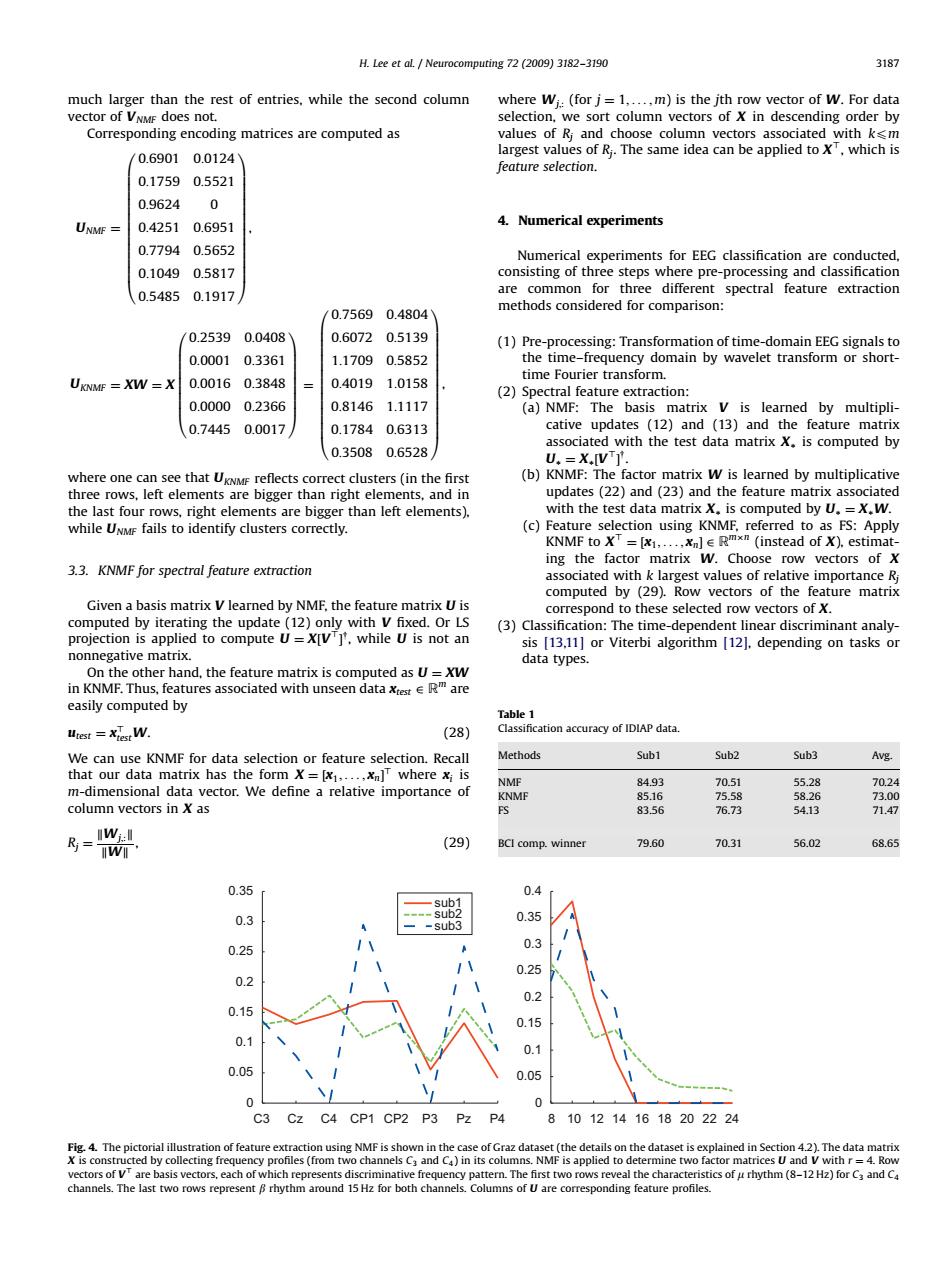
H.Lee et al.Neurocomputing 72 (2009)3182-3190 3187 much larger than the rest of entries,while the second column where Wi:(for j=1,....m)is the jth row vector of w.For data vector of VNMF does not. selection,we sort column vectors of X in descending order by Corresponding encoding matrices are computed as values of Ri and choose column vectors associated with ksm largest values of Ri.The same idea can be applied to X',which is 0.69010.0124 feature selection. 0.17590.5521 0.9624 0 UNMF 0.42510.6951 4.Numerical experiments 0.77940.5652 Numerical experiments for EEG classification are conducted, 0.1049 0.5817 consisting of three steps where pre-processing and classification 0.5485 0.1917 are common for three different spectral feature extraction 0.75690.4804 methods considered for comparison: 0.2539 0.0408 0.6072 0.5139 (1)Pre-processing:Transformation of time-domain EEG signals to 0.0001 0.3361 1.17090.5852 the time-frequency domain by wavelet transform or short- time Fourier transform. UKNMF XW =X 0.0016 0.3848 0.40191.0158 (2)Spectral feature extraction: 0.0000 0.2366 0.81461.1117 (a)NMF:The basis matrix V is learned by multipli- 0.7445 0.0017 0.17840.6313 cative updates (12)and (13)and the feature matrix associated with the test data matrix X.is computed by 0.35080.6528 U.=X.IVT. where one can see that UKNMF reflects correct clusters(in the first (b)KNMF:The factor matrix W is learned by multiplicative three rows,left elements are bigger than right elements,and in updates(22)and (23)and the feature matrix associated the last four rows,right elements are bigger than left elements). with the test data matrix X.is computed by U.=X.W. while UNME fails to identify clusters correctly. (c)Feature selection using KNMF,referred to as FS:Apply KNMF to XT =[x1,....xn]E Rmxm (instead of X).estimat- ing the factor matrix W.Choose row vectors of X 3.3.KNMF for spectral feature extraction associated with k largest values of relative importance Ri computed by (29).Row vectors of the feature matrix Given a basis matrix V learned by NMF,the feature matrix U is correspond to these selected row vectors of X. computed by iterating the update(12)only with V fixed.Or LS (3)Classification:The time-dependent linear discriminant analy- projection is applied to compute U=X[VT]'.while U is not an sis [13.11]or Viterbi algorithm [12].depending on tasks or nonnegative matrix. data types. On the other hand,the feature matrix is computed as U=XW in KNMF.Thus,features associated with unseen data xrest e Rare easily computed by Table 1 Utest =Xiest W. (28) Classification accuracy of IDIAP data. We can use KNMF for data selection or feature selection.Recall Methods Sub1 Sub2 Sub3 Avg. that our data matrix has the form X=[x1,...,xn]where x;is NMF 84.93 70.51 55.28 70.24 m-dimensional data vector.We define a relative importance of KNMF 85.16 75.58 58.26 73.00 column vectors in X as ES 83.56 76.73 54.13 71.47 号=w 70.31 56.02 I (29) BCI comp.winner 79.60 68.65 0.35 0.4 0.3 0.35 -sub3 0.25 0.3 0.25 0.2 0.2 0.15 0.15 0.1 0.1 0.05 0.05 0 0 C3 Cz C4 CP1 CP2 P3 Pz P4 8 1012141618202224 Fig.4.The pictorial illustration of feature extraction using NMF is shown in the case of Graz dataset(the details on the dataset is explained in Section 4.2).The data matrix r eve h mima pure Thethe hara(rndc channels.The last two rows represent B rhythm around 15 Hz for both channels.Columns of U are corresponding feature profiles.much larger than the rest of entries, while the second column vector of VNMF does not. Corresponding encoding matrices are computed as UNMF ¼ 0:6901 0:0124 0:1759 0:5521 0:9624 0 0:4251 0:6951 0:7794 0:5652 0:1049 0:5817 0:5485 0:1917 0 BBBBBBBBBBBBBB@ 1 CCCCCCCCCCCCCCA , UKNMF ¼ XW ¼ X 0:2539 0:0408 0:0001 0:3361 0:0016 0:3848 0:0000 0:2366 0:7445 0:0017 0 BBBBBBBB@ 1 CCCCCCCCA ¼ 0:7569 0:4804 0:6072 0:5139 1:1709 0:5852 0:4019 1:0158 0:8146 1:1117 0:1784 0:6313 0:3508 0:6528 0 BBBBBBBBBBBBBB@ 1 CCCCCCCCCCCCCCA , where one can see that UKNMF reflects correct clusters (in the first three rows, left elements are bigger than right elements, and in the last four rows, right elements are bigger than left elements), while UNMF fails to identify clusters correctly. 3.3. KNMF for spectral feature extraction Given a basis matrix V learned by NMF, the feature matrix U is computed by iterating the update (12) only with V fixed. Or LS projection is applied to compute U ¼ X½V> y , while U is not an nonnegative matrix. On the other hand, the feature matrix is computed as U ¼ XW in KNMF. Thus, features associated with unseen data xtest 2 Rm are easily computed by utest ¼ x> testW. (28) We can use KNMF for data selection or feature selection. Recall that our data matrix has the form X ¼ ½x1; ... ; xn > where xi is m-dimensional data vector. We define a relative importance of column vectors in X as Rj ¼ kWj;:k kWk , (29) where Wj;: (for j ¼ 1; ... ; m) is the jth row vector of W. For data selection, we sort column vectors of X in descending order by values of Rj and choose column vectors associated with kpm largest values of Rj. The same idea can be applied to X>, which is feature selection. 4. Numerical experiments Numerical experiments for EEG classification are conducted, consisting of three steps where pre-processing and classification are common for three different spectral feature extraction methods considered for comparison: (1) Pre-processing: Transformation of time-domain EEG signals to the time–frequency domain by wavelet transform or short￾time Fourier transform. (2) Spectral feature extraction: (a) NMF: The basis matrix V is learned by multipli￾cative updates (12) and (13) and the feature matrix associated with the test data matrix X is computed by U ¼ X½V> y . (b) KNMF: The factor matrix W is learned by multiplicative updates (22) and (23) and the feature matrix associated with the test data matrix X is computed by U ¼ XW. (c) Feature selection using KNMF, referred to as FS: Apply KNMF to X> ¼ ½x1; ... ; xn 2 Rmn (instead of X), estimat￾ing the factor matrix W. Choose row vectors of X associated with k largest values of relative importance Rj computed by (29). Row vectors of the feature matrix correspond to these selected row vectors of X. (3) Classification: The time-dependent linear discriminant analy￾sis [13,11] or Viterbi algorithm [12], depending on tasks or data types. ARTICLE IN PRESS Table 1 Classification accuracy of IDIAP data. Methods Sub1 Sub2 Sub3 Avg. NMF 84.93 70.51 55.28 70.24 KNMF 85.16 75.58 58.26 73.00 FS 83.56 76.73 54.13 71.47 BCI comp. winner 79.60 70.31 56.02 68.65 C3 0 0.05 0.1 0.15 0.2 0.25 0.3 0.35 sub1 sub2 sub3 8 0 0.05 0.1 0.15 0.2 0.25 0.3 0.35 0.4 Cz C4 CP1 CP2 P3 Pz P4 10 12 14 16 18 20 22 24 Fig. 4. The pictorial illustration of feature extraction using NMF is shown in the case of Graz dataset (the details on the dataset is explained in Section 4.2). The data matrix X is constructed by collecting frequency profiles (from two channels C3 and C4) in its columns. NMF is applied to determine two factor matrices U and V with r ¼ 4. Row vectors of V> are basis vectors, each of which represents discriminative frequency pattern. The first two rows reveal the characteristics of m rhythm (8–12 Hz) for C3 and C4 channels. The last two rows represent b rhythm around 15 Hz for both channels. Columns of U are corresponding feature profiles. H. Lee et al. / Neurocomputing 72 (2009) 3182–3190 3187