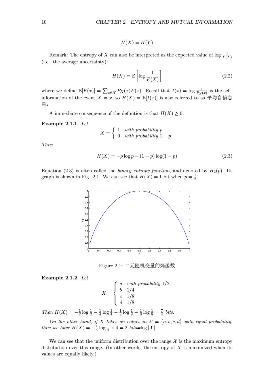
10 CHAPTER 2.ENTROPY AND MUTUAL INFORMATION H(X=H(Y) Remark:The entropy of can also be interpreted as the expected value of log (i.e,the average uncertainty）：片 H(X)=E108 P(X) 1 (2.2) where we define [F()F().Recall that I()og is the self formation of the event=,soH(X)=E[I(e月is also referred toas平均自信息 量 A immediate consequence of the definition is that H(X)>0. Example 2.1.1.Let 1 with mrobabilitu X=0 with probability 1-p Then H(X)=-plogp-(1-p)log(1-p) (2.3) )) 44 Figure2.1:二元随机变量的熵函数 Example 2.1.2.Let a with probability 1/2 X= 61/4 e1/8 d1/8 ThenH(X)=-log麦-log}-专log8-&log是=是bits. =fa,b,c,d}with equal probability, then we ha We can see tha the unif orm distr 10 CHAPTER 2. ENTROPY AND MUTUAL INFORMATION H(X) = H(Y ) Remark: The entropy of X can also be interpreted as the expected value of log 1 P(X) (i.e., the average uncertainty): H(X) = E [ log 1 P(X) ] (2.2) where we define E[F(x)] = ∑ x∈X PX(x)F(x). Recall that I(x) = log 1 PX(x) is the self￾information of the event X = x, so H(X) = E[I(x)] is also referred to as 平均自信息 量。 A immediate consequence of the definition is that H(X) ≥ 0. Example 2.1.1. Let X = { 1 with probability p 0 with probability 1 − p Then H(X) = −p log p − (1 − p) log(1 − p) (2.3) Equation (2.3) is often called the binary entropy function, and denoted by H2(p). Its graph is shown in Fig. 2.1. We can see that H(X) = 1 bit when p = 1 2 . 0 0.1 0.2 0.3 0.4 0.5 0.6 0.7 0.8 0.9 1 0 0.1 0.2 0.3 0.4 0.5 0.6 0.7 0.8 0.9 1 p H(p) Figure 2.1: 二元随机变量的熵函数 Example 2.1.2. Let X =    a with probability 1/2 b 1/4 c 1/8 d 1/8 Then H(X) = − 1 2 log 1 2 − 1 4 log 1 4 − 1 8 log 1 8 − 1 8 log 1 8 = 7 4 bits. On the other hand, if X takes on values in X = {a, b, c, d} with equal probability, then we have H(X) = − 1 4 log 1 4 × 4 = 2 bits=log |X |. We can see that the uniform distribution over the range X is the maximum entropy distribution over this range. (In other words, the entropy of X is maximized when its values are equally likely.)