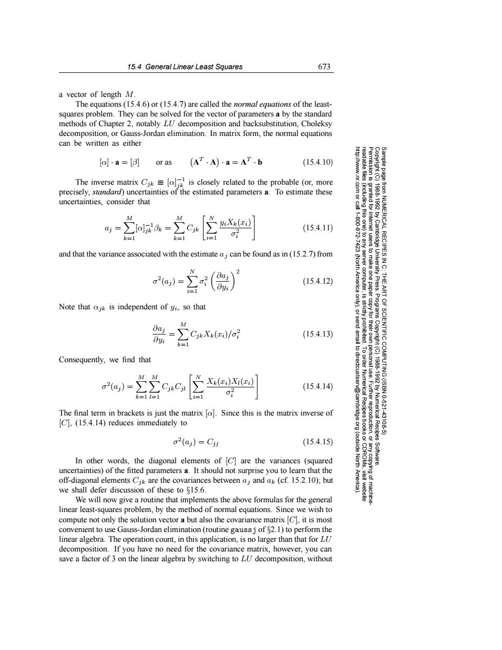
15.4 General Linear Least Squares 673 a vector of length M. The equations (15.4.6)or(15.4.7)are called the normal equations of the least- squares problem.They can be solved for the vector of parameters a by the standard methods of Chapter 2,notably LU decomposition and backsubstitution,Choleksy decomposition,or Gauss-Jordan elimination.In matrix form,the normal equations can be written as either [al·a=[例 or as (AT.A)·a=AT.b (15.4.10) The inverse matrix C is closely related to the probable (or,more precisely,standard)uncertainties of the estimated parameters a.To estimate these uncertainties,consider that M ∑aR=∑C 02 (15.4.11) and that the variance associated with the estimate a;can be found as in (15.2.7)from RECIPES 令 2(a） ∑ (15.4.12) Press. Note that ajk is independent of yi,so that 9 M =CjkXx(1)/o? (15.4.13) 0班 IENTIFIC k=1 6 Consequently,we find that o2(aj) Xk(zi)XI(xi) 15.4.14) k=1= The final term in brackets is just the matrix [a].Since this is the matrix inverse of Numerical 105211 [C],(15.4.14)reduces immediately to 431 a2(a）=C7 (15.4.15) (outside Recipes In other words,the diagonal elements of [C]are the variances (squared North uncertainties)of the fitted parameters a.It should not surprise you to learn that the off-diagonal elements Cik are the covariances between a;and ak(cf.15.2.10);but we shall defer discussion of these to 815.6. We will now give a routine that implements the above formulas for the general linear least-squares problem,by the method of normal equations.Since we wish to compute not only the solution vector a but also the covariance matrix [C],it is most convenient to use Gauss-Jordan elimination(routine gaussj of 82.1)to perform the linear algebra.The operation count,in this application,is no larger than that for LU decomposition.If you have no need for the covariance matrix,however,you can save a factor of 3 on the linear algebra by switching to LU decomposition,without15.4 General Linear Least Squares 673 Permission is granted for internet users to make one paper copy for their own personal use. Further reproduction, or any copyin Copyright (C) 1988-1992 by Cambridge University Press. Programs Copyright (C) 1988-1992 by Numerical Recipes Software. Sample page from NUMERICAL RECIPES IN C: THE ART OF SCIENTIFIC COMPUTING (ISBN 0-521-43108-5) g of machine￾readable files (including this one) to any server computer, is strictly prohibited. To order Numerical Recipes books or CDROMs, visit website http://www.nr.com or call 1-800-872-7423 (North America only), or send email to directcustserv@cambridge.org (outside North America). a vector of length M. The equations (15.4.6) or (15.4.7) are called the normal equations of the least￾squares problem. They can be solved for the vector of parameters a by the standard methods of Chapter 2, notably LU decomposition and backsubstitution, Choleksy decomposition, or Gauss-Jordan elimination. In matrix form, the normal equations can be written as either [α] · a = [β] or as AT · A · a = AT · b (15.4.10) The inverse matrix Cjk ≡ [α] −1 jk is closely related to the probable (or, more precisely, standard) uncertainties of the estimated parameters a. To estimate these uncertainties, consider that aj =
M k=1 [α] −1 jk βk =
M k=1 Cjk
N i=1 yiXk(xi) σ2 i  (15.4.11) and that the variance associated with the estimate aj can be found as in (15.2.7) from σ2(aj ) =
N i=1 σ2 i ∂aj ∂yi 2 (15.4.12) Note that αjk is independent of yi, so that ∂aj ∂yi =
M k=1 CjkXk(xi)/σ2 i (15.4.13) Consequently, we find that σ2(aj ) =
M k=1
M l=1 CjkCjl
N i=1 Xk(xi)Xl(xi) σ2 i  (15.4.14) The final term in brackets is just the matrix [α]. Since this is the matrix inverse of [C], (15.4.14) reduces immediately to σ2(aj ) = Cjj (15.4.15) In other words, the diagonal elements of [C] are the variances (squared uncertainties) of the fitted parameters a. It should not surprise you to learn that the off-diagonal elements Cjk are the covariances between aj and ak (cf. 15.2.10); but we shall defer discussion of these to §15.6. We will now give a routine that implements the above formulas for the general linear least-squares problem, by the method of normal equations. Since we wish to compute not only the solution vector a but also the covariance matrix [C], it is most convenient to use Gauss-Jordan elimination (routine gaussj of §2.1) to perform the linear algebra. The operation count, in this application, is no larger than that for LU decomposition. If you have no need for the covariance matrix, however, you can save a factor of 3 on the linear algebra by switching to LU decomposition, without