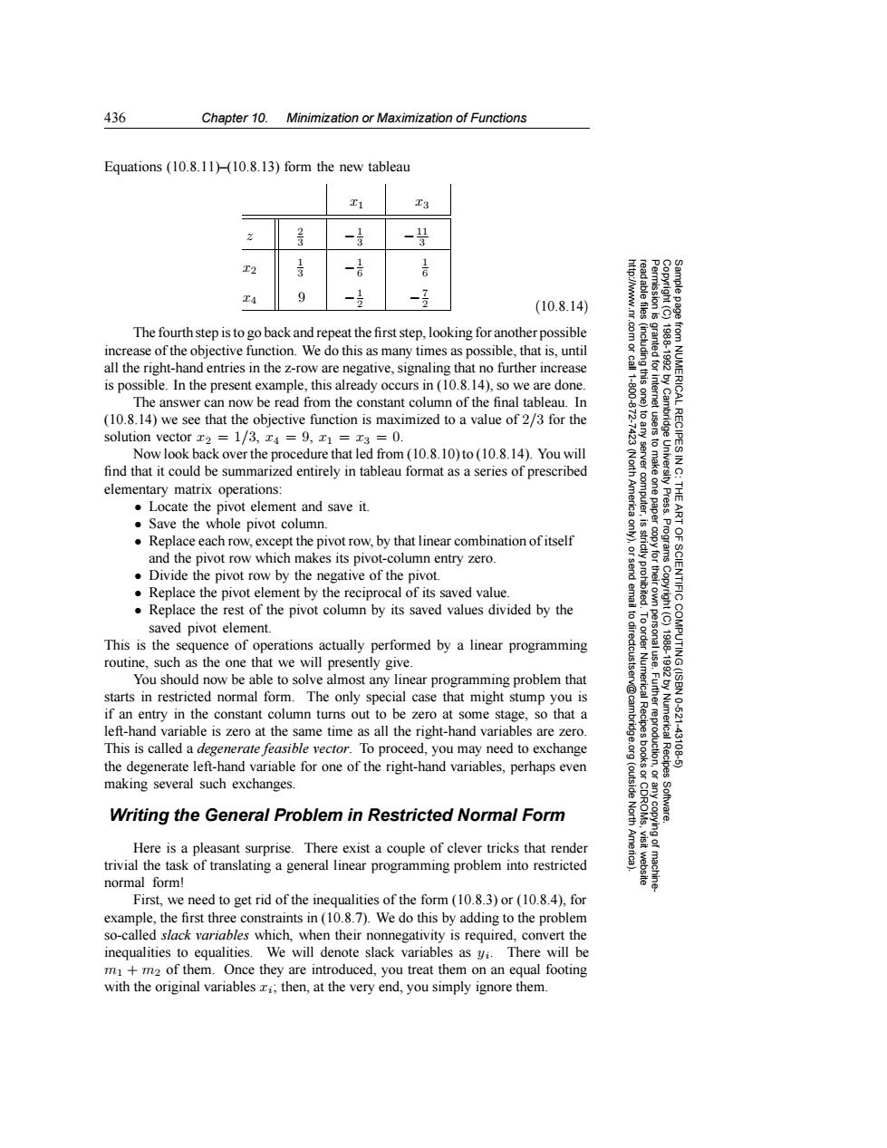
436 Chapter 10. Minimization or Maximization of Functions Equations (10.8.11)-(10.8.13)form the new tableau T1 3 2 23 一 -号 工2 13 -君 吉 TA 9 一 (10.8.14) The fourth step is to go back and repeat the first step,looking for another possible increase of the objective function.We do this as many times as possible,that is,until all the right-hand entries in the z-row are negative,signaling that no further increase nted for is possible.In the present example,this already occurs in(10.8.14),so we are done. The answer can now be read from the constant column of the final tableau.In (10.8.14)we see that the objective function is maximized to a value of 2/3 for the solution vector 2 1/3,x4 9,x1 x3 =0. RECIPES I Now look back over the procedure that led from(10.8.10)to (10.8.14).You will 令 find that it could be summarized entirely in tableau format as a series of prescribed elementary matrix operations: Locate the pivot element and save it. p Press. Save the whole pivot column. Replace each row,except the pivot row,by that linear combination ofitself and the pivot row which makes its pivot-column entry zero Divide the pivot row by the negative of the pivot. Replace the pivot element by the reciprocal of its saved value SCIENTIFIC Replace the rest of the pivot column by its saved values divided by the saved pivot element. to dir This is the sequence of operations actually performed by a linear programming routine,such as the one that we will presently give. You should now be able to solve almost any linear programming problem that starts in restricted normal form.The only special case that might stump you is if an entry in the constant column turns out to be zero at some stage,so that a Recipes Numerical Recipes 10.621 left-hand variable is zero at the same time as all the right-hand variables are zero. This is called a degenerate feasible vector.To proceed,you may need to exchange E喜 43106 the degenerate left-hand variable for one of the right-hand variables,perhaps even making several such exchanges. 腿 Writing the General Problem in Restricted Normal Form North Here is a pleasant surprise.There exist a couple of clever tricks that render trivial the task of translating a general linear programming problem into restricted normal form! First,we need to get rid of the inequalities of the form (10.8.3)or (10.8.4).for example,the first three constraints in (10.8.7).We do this by adding to the problem so-called slack variables which,when their nonnegativity is required,convert the inequalities to equalities.We will denote slack variables as yi.There will be m+m2 of them.Once they are introduced,you treat them on an equal footing with the original variables zi;then,at the very end,you simply ignore them.436 Chapter 10. Minimization or Maximization of Functions Permission is granted for internet users to make one paper copy for their own personal use. Further reproduction, or any copyin Copyright (C) 1988-1992 by Cambridge University Press. Programs Copyright (C) 1988-1992 by Numerical Recipes Software. Sample page from NUMERICAL RECIPES IN C: THE ART OF SCIENTIFIC COMPUTING (ISBN 0-521-43108-5) g of machine￾readable files (including this one) to any server computer, is strictly prohibited. To order Numerical Recipes books or CDROMs, visit website http://www.nr.com or call 1-800-872-7423 (North America only), or send email to directcustserv@cambridge.org (outside North America). Equations (10.8.11)–(10.8.13) form the new tableau x1 x3 z 2 3 −1 3 −11 3 x2 1 3 −1 6 1 6 x4 9 −1 2 −7 2 (10.8.14) The fourth step is to go back and repeat the first step, looking for another possible increase of the objective function. We do this as many times as possible, that is, until all the right-hand entries in the z-row are negative, signaling that no further increase is possible. In the present example, this already occurs in (10.8.14), so we are done. The answer can now be read from the constant column of the final tableau. In (10.8.14) we see that the objective function is maximized to a value of 2/3 for the solution vector x2 = 1/3, x4 = 9, x1 = x3 = 0. Now look back over the procedure that led from (10.8.10) to (10.8.14). You will find that it could be summarized entirely in tableau format as a series of prescribed elementary matrix operations: • Locate the pivot element and save it. • Save the whole pivot column. • Replace each row, except the pivot row, by that linear combination of itself and the pivot row which makes its pivot-column entry zero. • Divide the pivot row by the negative of the pivot. • Replace the pivot element by the reciprocal of its saved value. • Replace the rest of the pivot column by its saved values divided by the saved pivot element. This is the sequence of operations actually performed by a linear programming routine, such as the one that we will presently give. You should now be able to solve almost any linear programming problem that starts in restricted normal form. The only special case that might stump you is if an entry in the constant column turns out to be zero at some stage, so that a left-hand variable is zero at the same time as all the right-hand variables are zero. This is called a degenerate feasible vector. To proceed, you may need to exchange the degenerate left-hand variable for one of the right-hand variables, perhaps even making several such exchanges. Writing the General Problem in Restricted Normal Form Here is a pleasant surprise. There exist a couple of clever tricks that render trivial the task of translating a general linear programming problem into restricted normal form! First, we need to get rid of the inequalities of the form (10.8.3) or (10.8.4), for example, the first three constraints in (10.8.7). We do this by adding to the problem so-called slack variables which, when their nonnegativity is required, convert the inequalities to equalities. We will denote slack variables as yi. There will be m1 + m2 of them. Once they are introduced, you treat them on an equal footing with the original variables xi; then, at the very end, you simply ignore them