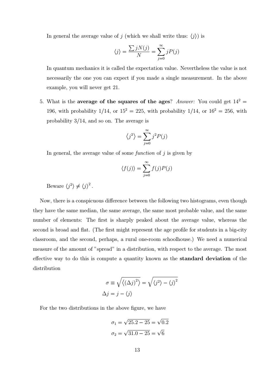
In general the average value of j(which we shall write thus:(j))is 0=2N0-2P60) 0 In quantum mechanics it is called the expectation value.Nevertheless the value is not necessarily the one you can expect if you made a single measurement.In the above example,you will never get 21 5.What is the average of the squares of the ages?Answer:You could get 142- 196,with probability 1/14,or 152=225,with probability 1/14,or 162=256,with probability 3/14,and so on.The average is G)=-∑P0) j= In general,the average value of some function of j is given by G=∑fG)PO) Beware(2)≠) Now,there is a conspicuous difference between the following two histograms,even though they have the same median,the same average,the same most probable value,and the same number of elements:The first is sharply peaked about the average value,whereas the second is broad and flat.(The first might represent the age profile for students in a big-city classroom,and the second,perhaps,a rural one-room schoolhouse.)We need a numerical measure of the amount of"spread"in a distribution,with respect to the average.The most effective way to do this is compute a quantity known as the standard deviation of the distribution σ三V(A)2〉=VG)-》 △=j-》 For the two distributions in the above figure,we have 01=V25.2-25=V0.2 02=V31.0-25=V6 13In general the average value of j (which we shall write thus: hji) is hji = PjN(j) N = X∞ j=0 jP(j) In quantum mechanics it is called the expectation value. Nevertheless the value is not necessarily the one you can expect if you made a single measurement. In the above example, you will never get 21. 5. What is the average of the squares of the ages? Answer: You could get 142 = 196, with probability 1/14, or 152 = 225, with probability 1/14, or 162 = 256, with probability 3/14, and so on. The average is ­ j 2 ® = X∞ j=0 j 2P(j) In general, the average value of some function of j is given by hf(j)i = X∞ j=0 f(j)P(j) Beware hj 2 i 6= hji 2 . Now, there is a conspicuous difference between the following two histograms, even though they have the same median, the same average, the same most probable value, and the same number of elements: The first is sharply peaked about the average value, whereas the second is broad and flat. (The first might represent the age profile for students in a big-city classroom, and the second, perhaps, a rural one-room schoolhouse.) We need a numerical measure of the amount of ”spread” in a distribution, with respect to the average. The most effective way to do this is compute a quantity known as the standard deviation of the distribution σ ≡ q­ (∆j) 2 ® = q hj 2i − hji 2 ∆j = j − hji For the two distributions in the above figure, we have σ1 = √ 25.2 − 25 = √ 0.2 σ2 = √ 31.0 − 25 = √ 6 13