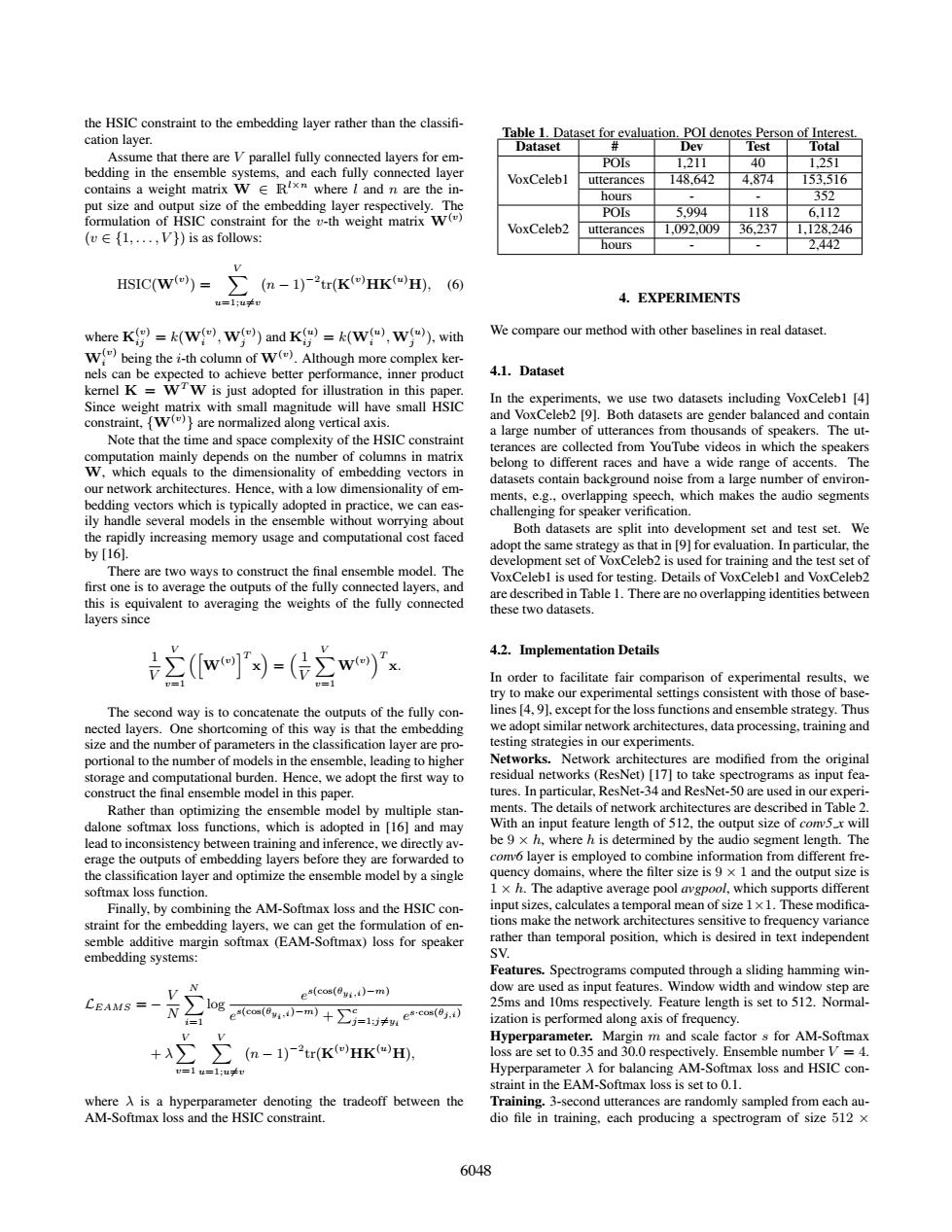
the HSIC constraint to the embedding layer rather than the classifi- cation layer. Table 1.Dataset for evaluation.POI denotes Person of Interest. Dataset # Dev Test Total Assume that there are V parallel fully connected layers for em- POIs 1.211 40 1,25I bedding in the ensemble systems,and each fully connected layer VoxCeleb1 utterances 148.642 4.874 153.516 contains a weight matrix W E R'xm where I and n are the in- hours 352 put size and output size of the embedding layer respectively.The formulation of HSIC constraint for the v-th weight matrix W() POIs 5.994 118 6,112 VoxCeleb2 utterances 1.092.00936.237 1.128.246 (u∈{1，..，V})is as follows: hours 2.442 HSIC(W())=>(n-1)-2tr(K()HK()H),(6) u=1u≠知 4.EXPERIMENTS where K(=W(),W())and K()=k(W(),W()).with We compare our method with other baselines in real dataset W)being the i-th column of W().Although more complex ker- nels can be expected to achieve better performance,inner product 4.1.Dataset kerel K =WTW is just adopted for illustration in this paper. In the experiments,we use two datasets including VoxCelebl [4) Since weight matrix with small magnitude will have small HSIC constraint,{W()}are normalized along vertical axis. and VoxCeleb2 [9].Both datasets are gender balanced and contain a large number of utterances from thousands of speakers.The ut- Note that the time and space complexity of the HSIC constraint terances are collected from YouTube videos in which the speakers computation mainly depends on the number of columns in matrix belong to different races and have a wide range of accents.The W.which equals to the dimensionality of embedding vectors in datasets contain background noise from a large number of environ- our network architectures.Hence,with a low dimensionality of em- bedding vectors which is typically adopted in practice,we can eas- ments,e.g.,overlapping speech,which makes the audio segments ily handle several models in the ensemble without worrying about challenging for speaker verification. the rapidly increasing memory usage and computational cost faced Both datasets are split into development set and test set.We adopt the same strategy as that in [9]for evaluation.In particular,the by[16. development set of VoxCeleb2 is used for training and the test set of There are two ways to construct the final ensemble model.The VoxCelebl is used for testing.Details of VoxCelebl and VoxCeleb2 first one is to average the outputs of the fully connected layers,and are described in Table 1.There are no overlapping identities between this is equivalent to averaging the weights of the fully connected hese two datasets. layers since 4.2.Implementation Details ∑(w]'x=(∑w)x In order to facilitate fair comparison of experimental results,we try to make our experimental settings consistent with those of base- The second way is to concatenate the outputs of the fully con- lines [4,9],except for the loss functions and ensemble strategy.Thus nected layers.One shortcoming of this way is that the embedding we adopt similar network architectures,data processing,training and size and the number of parameters in the classification layer are pro- testing strategies in our experiments. portional to the number of models in the ensemble,leading to higher Networks.Network architectures are modified from the original storage and computational burden.Hence,we adopt the first way to residual networks (ResNet)[17]to take spectrograms as input fea- construct the final ensemble model in this paper. tures.In particular,ResNet-34 and ResNet-50 are used in our experi- Rather than optimizing the ensemble model by multiple stan- ments.The details of network architectures are described in Table 2. dalone softmax loss functions,which is adopted in [16]and may With an input feature length of 512,the output size of com5_x will lead to inconsistency between training and inference,we directly av- be 9 x h,where h is determined by the audio segment length.The erage the outputs of embedding layers before they are forwarded to cono layer is employed to combine information from different fre- the classification layer and optimize the ensemble model by a single quency domains,where the filter size is 9 x 1 and the output size is softmax loss function. 1x h.The adaptive average pool avgpool,which supports different Finally,by combining the AM-Softmax loss and the HSIC con- input sizes,calculates a temporal mean of size 1x 1.These modifica- straint for the embedding layers,we can get the formulation of en- tions make the network architectures sensitive to frequency variance semble additive margin softmax (EAM-Softmax)loss for speaker rather than temporal position,which is desired in text independent embedding systems: SV. Features.Spectrograms computed through a sliding hamming win- es(cos(0vi.i)-m) dow are used as input features.Window width and window step are CEAMS=- ∑og 25ms and 10ms respectively.Feature length is set to 512.Normal- i三1 (co(v)-m)eco() ization is performed along axis of frequency. Hyperparameter.Margin m and scale factor s for AM-Softmax +λ(m-1)-2tr(KHK(H) loss are set to 0.35 and 30.0 respectively.Ensemble number V =4. =1 u=1:u≠t Hyperparameter A for balancing AM-Softmax loss and HSIC con- straint in the EAM-Softmax loss is set to 0.1. where A is a hyperparameter denoting the tradeoff between the Training.3-second utterances are randomly sampled from each au- AM-Softmax loss and the HSIC constraint. dio file in training,each producing a spectrogram of size 512 x 6048the HSIC constraint to the embedding layer rather than the classifi- cation layer. Assume that there are V parallel fully connected layers for em￾bedding in the ensemble systems, and each fully connected layer contains a weight matrix W ∈ R l×n where l and n are the in￾put size and output size of the embedding layer respectively. The formulation of HSIC constraint for the v-th weight matrix W(v) (v ∈ {1, . . . , V }) is as follows: HSIC(W(v) ) = XV u=1;u6=v (n − 1)−2 tr(K (v)HK(u)H), (6) where K (v) ij = k(W(v) i ,W(v) j ) and K (u) ij = k(W(u) i ,W(u) j ), with W(v) i being the i-th column of W(v) . Although more complex ker￾nels can be expected to achieve better performance, inner product kernel K = WTW is just adopted for illustration in this paper. Since weight matrix with small magnitude will have small HSIC constraint, {W(v) } are normalized along vertical axis. Note that the time and space complexity of the HSIC constraint computation mainly depends on the number of columns in matrix W, which equals to the dimensionality of embedding vectors in our network architectures. Hence, with a low dimensionality of em￾bedding vectors which is typically adopted in practice, we can eas￾ily handle several models in the ensemble without worrying about the rapidly increasing memory usage and computational cost faced by [16]. There are two ways to construct the final ensemble model. The first one is to average the outputs of the fully connected layers, and this is equivalent to averaging the weights of the fully connected layers since 1 V XV v=1 hW(v) iT x  =  1 V XV v=1 W(v) T x. The second way is to concatenate the outputs of the fully con￾nected layers. One shortcoming of this way is that the embedding size and the number of parameters in the classification layer are pro￾portional to the number of models in the ensemble, leading to higher storage and computational burden. Hence, we adopt the first way to construct the final ensemble model in this paper. Rather than optimizing the ensemble model by multiple stan￾dalone softmax loss functions, which is adopted in [16] and may lead to inconsistency between training and inference, we directly av￾erage the outputs of embedding layers before they are forwarded to the classification layer and optimize the ensemble model by a single softmax loss function. Finally, by combining the AM-Softmax loss and the HSIC con￾straint for the embedding layers, we can get the formulation of en￾semble additive margin softmax (EAM-Softmax) loss for speaker embedding systems: LEAMS = − V N XN i=1 log e s(cos(θyi ,i)−m) e s(cos(θyi ,i)−m) + Pc j=1;j6=yi e s·cos(θj,i) + λ XV v=1 XV u=1;u6=v (n − 1)−2 tr(K (v)HK(u)H), where λ is a hyperparameter denoting the tradeoff between the AM-Softmax loss and the HSIC constraint. Table 1. Dataset for evaluation. POI denotes Person of Interest. Dataset # Dev Test Total VoxCeleb1 POIs 1,211 40 1,251 utterances 148,642 4,874 153,516 hours - - 352 VoxCeleb2 POIs 5,994 118 6,112 utterances 1,092,009 36,237 1,128,246 hours - - 2,442 4. EXPERIMENTS We compare our method with other baselines in real dataset. 4.1. Dataset In the experiments, we use two datasets including VoxCeleb1 [4] and VoxCeleb2 [9]. Both datasets are gender balanced and contain a large number of utterances from thousands of speakers. The ut￾terances are collected from YouTube videos in which the speakers belong to different races and have a wide range of accents. The datasets contain background noise from a large number of environ￾ments, e.g., overlapping speech, which makes the audio segments challenging for speaker verification. Both datasets are split into development set and test set. We adopt the same strategy as that in [9] for evaluation. In particular, the development set of VoxCeleb2 is used for training and the test set of VoxCeleb1 is used for testing. Details of VoxCeleb1 and VoxCeleb2 are described in Table 1. There are no overlapping identities between these two datasets. 4.2. Implementation Details In order to facilitate fair comparison of experimental results, we try to make our experimental settings consistent with those of base￾lines [4, 9], except for the loss functions and ensemble strategy. Thus we adopt similar network architectures, data processing, training and testing strategies in our experiments. Networks. Network architectures are modified from the original residual networks (ResNet) [17] to take spectrograms as input fea￾tures. In particular, ResNet-34 and ResNet-50 are used in our experi￾ments. The details of network architectures are described in Table 2. With an input feature length of 512, the output size of conv5 x will be 9 × h, where h is determined by the audio segment length. The conv6 layer is employed to combine information from different fre￾quency domains, where the filter size is 9 × 1 and the output size is 1 × h. The adaptive average pool avgpool, which supports different input sizes, calculates a temporal mean of size 1×1. These modifica￾tions make the network architectures sensitive to frequency variance rather than temporal position, which is desired in text independent SV. Features. Spectrograms computed through a sliding hamming win￾dow are used as input features. Window width and window step are 25ms and 10ms respectively. Feature length is set to 512. Normal￾ization is performed along axis of frequency. Hyperparameter. Margin m and scale factor s for AM-Softmax loss are set to 0.35 and 30.0 respectively. Ensemble number V = 4. Hyperparameter λ for balancing AM-Softmax loss and HSIC con￾straint in the EAM-Softmax loss is set to 0.1. Training. 3-second utterances are randomly sampled from each au￾dio file in training, each producing a spectrogram of size 512 × 6048