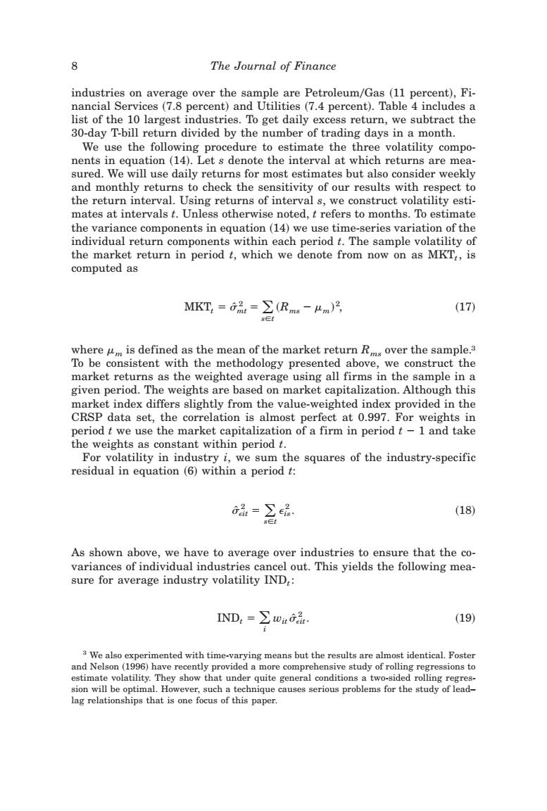
8 The Journal of Finance industries on average over the sample are Petroleum/Gas (11 percent),Fi- nancial Services (7.8 percent)and Utilities(7.4 percent).Table 4 includes a list of the 10 largest industries.To get daily excess return,we subtract the 30-day T-bill return divided by the number of trading days in a month. We use the following procedure to estimate the three volatility compo- nents in equation(14).Let s denote the interval at which returns are mea- sured.We will use daily returns for most estimates but also consider weekly and monthly returns to check the sensitivity of our results with respect to the return interval.Using returns of interval s,we construct volatility esti- mates at intervals t.Unless otherwise noted,t refers to months.To estimate the variance components in equation(14)we use time-series variation of the individual return components within each period t.The sample volatility of the market return in period t,which we denote from now on as MKT,is computed as MKT=G品=∑(Rm-um)2 (17) sEt where um is defined as the mean of the market return R over the sample.s To be consistent with the methodology presented above,we construct the market returns as the weighted average using all firms in the sample in a given period.The weights are based on market capitalization.Although this market index differs slightly from the value-weighted index provided in the CRSP data set,the correlation is almost perfect at 0.997.For weights in period t we use the market capitalization of a firm in period t-1 and take the weights as constant within period t. For volatility in industry i,we sum the squares of the industry-specific residual in equation(6)within a period t: 品-∑品. (18) s∈t As shown above,we have to average over industries to ensure that the co- variances of individual industries cancel out.This yields the following mea- sure for average industry volatility IND,: ND,=∑wtG品. (19) 3 We also experimented with time-varying means but the results are almost identical.Foster and Nelson(1996)have recently provided a more comprehensive study of rolling regressions to estimate volatility.They show that under quite general conditions a two-sided rolling regres- sion will be optimal.However,such a technique causes serious problems for the study of lead- lag relationships that is one focus of this paper.industries on average over the sample are Petroleum0Gas ~11 percent!, Fi￾nancial Services ~7.8 percent! and Utilities ~7.4 percent!. Table 4 includes a list of the 10 largest industries. To get daily excess return, we subtract the 30-day T-bill return divided by the number of trading days in a month. We use the following procedure to estimate the three volatility compo￾nents in equation ~14!. Let s denote the interval at which returns are mea￾sured. We will use daily returns for most estimates but also consider weekly and monthly returns to check the sensitivity of our results with respect to the return interval. Using returns of interval s, we construct volatility esti￾mates at intervals t. Unless otherwise noted, t refers to months. To estimate the variance components in equation ~14! we use time-series variation of the individual return components within each period t. The sample volatility of the market return in period t, which we denote from now on as MKTt, is computed as MKTt 5 s[ mt 2 5 (s[t ~Rms 2 mm!2 , ~17! where mm is defined as the mean of the market return Rms over the sample.3 To be consistent with the methodology presented above, we construct the market returns as the weighted average using all firms in the sample in a given period. The weights are based on market capitalization. Although this market index differs slightly from the value-weighted index provided in the CRSP data set, the correlation is almost perfect at 0.997. For weights in period t we use the market capitalization of a firm in period t 2 1 and take the weights as constant within period t. For volatility in industry i, we sum the squares of the industry-specific residual in equation ~6! within a period t: s[ eit 2 5 (s[t eis 2 . ~18! As shown above, we have to average over industries to ensure that the co￾variances of individual industries cancel out. This yields the following mea￾sure for average industry volatility INDt: INDt 5 ( i wit s[ eit 2 . ~19! 3 We also experimented with time-varying means but the results are almost identical. Foster and Nelson ~1996! have recently provided a more comprehensive study of rolling regressions to estimate volatility. They show that under quite general conditions a two-sided rolling regres￾sion will be optimal. However, such a technique causes serious problems for the study of lead– lag relationships that is one focus of this paper. 8 The Journal of Finance