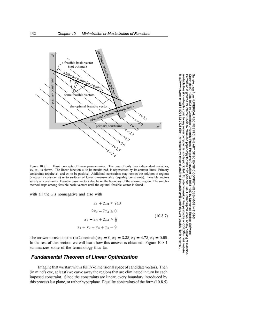
432 Chapter 10. Minimization or Maximization of Functions a feasible basic vector (not optimal) additional con additional constraint(equality) aint 个 (inequal http://www.nr. Permission is readable files some feasible vectors granted fori the optimal feasible vector inequality） (including this one) additional constraint =3.1 .com or call 1-800-872- primary constraint =2.9 from NUMERICAL RECIPES IN X2 2=2.8 2=2.7 2=2.6 (North America to any server computer, tusers to make one paper 1988-1992 by Cambridge University Press. THE 2=2.5 ART 2=2.4 是 Programs copy for their Figure 10.8.1.Basic concepts of linear programming. The case of only two independent variables, strictly prohibited c1,2,is shown.The linear function z,to be maximized,is represented by its contour lines.Primary constraints require c1 and r2 to be positive.Additional constraints may restrict the solution to regions (inequality constraints)or to surfaces of lower dimensionality (equality constraints).Feasible vectors to dir satisfy all constraints.Feasible basic vectors also lie on the boundary of the allowed region.The simplex method steps among feasible basic vectors until the optimal feasible vector is found. OF SCIENTIFIC COMPUTING (ISBN with all the z's nonnegative and also with 1788-1982 x1+2x3≤740 10-621 2x2-7x4≤0 .Further reproduction, 43108 (10.8.7) Numerical Recipes x2-x3+2x4≥ E1十r2+x3+E4=9 (outside North Software. The answer turns out to be (to 2 decimals)1=0,x2 =3.33,x3 =4.73,x4 =0.95. In the rest of this section we will learn how this answer is obtained.Figure 10.8.1 Ame summarizes some of the terminology thus far. visit website machine Fundamental Theorem of Linear Optimization Imagine that we start with a full N-dimensional space of candidate vectors.Then (in mind's eye,at least)we carve away the regions that are eliminated in turn by each imposed constraint.Since the constraints are linear,every boundary introduced by this process is a plane,or rather hyperplane.Equality constraints of the form(10.8.5)432 Chapter 10. Minimization or Maximization of Functions Permission is granted for internet users to make one paper copy for their own personal use. Further reproduction, or any copyin Copyright (C) 1988-1992 by Cambridge University Press. Programs Copyright (C) 1988-1992 by Numerical Recipes Software. Sample page from NUMERICAL RECIPES IN C: THE ART OF SCIENTIFIC COMPUTING (ISBN 0-521-43108-5) g of machine￾readable files (including this one) to any server computer, is strictly prohibited. To order Numerical Recipes books or CDROMs, visit website http://www.nr.com or call 1-800-872-7423 (North America only), or send email to directcustserv@cambridge.org (outside North America). additional constraint (inequality) additional constraint (inequality) the optimal feasible vector some feasible vectors x1 primary constraint x2 a feasible basic vector (not optimal) primary constraint additional constraint (equality) z = 3.1 z = 2.9 z = 2.8 z = 2.7 z = 2.6 z = 2.5 z = 2.4 z = 3.0 Figure 10.8.1. Basic concepts of linear programming. The case of only two independent variables, x1, x2, is shown. The linear function z, to be maximized, is represented by its contour lines. Primary constraints require x1 and x2 to be positive. Additional constraints may restrict the solution to regions (inequality constraints) or to surfaces of lower dimensionality (equality constraints). Feasible vectors satisfy all constraints. Feasible basic vectors also lie on the boundary of the allowed region. The simplex method steps among feasible basic vectors until the optimal feasible vector is found. with all the x’s nonnegative and also with x1 + 2x3 ≤ 740 2x2 − 7x4 ≤ 0 x2 − x3 + 2x4 ≥ 1 2 x1 + x2 + x3 + x4 = 9 (10.8.7) The answer turns out to be (to 2 decimals) x1 = 0, x2 = 3.33, x3 = 4.73, x4 = 0.95. In the rest of this section we will learn how this answer is obtained. Figure 10.8.1 summarizes some of the terminology thus far. Fundamental Theorem of Linear Optimization Imagine that we start with a full N-dimensional space of candidate vectors. Then (in mind’s eye, at least) we carve away the regions that are eliminated in turn by each imposed constraint. Since the constraints are linear, every boundary introduced by this process is a plane, or rather hyperplane. Equality constraints of the form (10.8.5)