Algorithm 1 Optimizing U using surrogate algorithm Input:XERNXD,S={s},Q,T∈N+,B,e∈Rt, Initializing U by performing PCA on X. fort=1→Tdo fori=1→Ndo Update Ui by following the rule given in (4). end for Compute L in(2)using the updated U. (a)Full (b)Sparse (c)Aligned Terminate the iterative process when the change of L is smaller than e. end for Figure 1:Selection of S for stochastic learning. Output:U∈RNxQ. 2.5 Stochastic Learning For a given set of N training points with supervised infor- 2.3.2 Out-of-Sample Extension mation,there are N x N pairs of similarity labels available In order to perform ANN search,we need to compute the to form S.Straightforwardly,we can choose S to include binary code b for a query x which is not in the training set. all the available similarity pairs,that is,S={s i,j= We achieve this by finding a matrix WRx that maps 1,...,N,i.This is illustrated in Figure 1(a),in which x to u in the following way: a colored cell in the i-th row and j-th column indicates that u=WTx. sij is included in S.In this way,the best possible accuracy can be achieved since we use as much as available semantic We then perform the same rounding technique discussed in information.However,according to the complexity analy- Section 2.3.1 on u to obtain b sis described in Section 2.4,if we set S to contain the full We use linear regression to train W over the training set supervised information,the time cost to update U would The squared loss with regularization term is shown below: become O(NQ3+N2Q2)per iteration,and O(N2)memory is needed to store S.Such cost in both computation and Le=IU-XW+入IW storage is unacceptable when N grows large. Inspired by stochastic gradient descent method,we pro And the optimal W can be computed as: pose an efficient way of updating U,called stochastic learn- W=(XX+AI)-xTU (5) ing.As illustrated in Figure 1(b),S contains a sparse subset with only O(NQ)entries which are randomly selected from 2.4 Convergence and Complexity Analysis all the available similarity pairs.The random sampling is performed for each iteration.We choose the size of S to At each iteration,we first construct a lower bound at the be O(NQ)so that the time cost to update U is reduced to current point Ui(t),and then optimize it to get a new point Ui(t+1)with a higher function value L(Uis(t+1)) O(NQ)per iteration.For storage efficiency,we compute only the sampled subset during each iteration.By this way Hence,the objective function value always increases in the the maximum required storage reduces to O(NQ) new iteration.Furthermore,the objective function value L=logp(U S)is upper bounded by zero.Hence,our Al- We can even further reduce the time cost by sampling S in an aligned way.During each iteration,an index set gorithm 1 can always guarantee convergence to local maxi- mum.the principle of which is similar to that of EM algo- I of size O(Q)is randomly chosen from {1,...,N}.We then construct S by using the rows and columns in Z,with rithm.This convergence property will also be illustrated in entries at the diagonal excluded.The resulted S is shown in Figure 2.The convergence property of our surrogate algo- Figure 1(c).Following this,the constructed S is guaranteed rithm is one of the key advantages compared with standard to be symmetric,and H;defined in (3)can be simplified as: Newton method and first-order gradient method.In both Newton method and first-order gradient method,a step size, 1 H;=- also called learning rate in some literatures,should be man- 8 ∑u ually specified,which cannot necessarily guarantee conver- gence. For all i the set fi:sii S}is exactly the same We can prove that,when updating Uis,the total time to thanks to the alignment of S.This implies that H;remains compute aL/aU.and Hi for all i 1,....N is (IS|Q) the same for all iZ.Therefore,we can compute H.in a and O(SQ),respectively.Since the inversion of Hi can be preprocessing step.By doing so,the time cost to update Uis computed in O(Q),the time to update U:s following the for each iI can be reduced to (Q-).For each iEI,we rule given in (4)is O(Q).Then the time to update U by can update Ui.through some complicated calculations while one iteration is O(NQ+SQ2).Therefore,the total time still maintaining the (Q2)time complexity.We can also of the updating process is O(T(NO+SQ)),where T is safely skip updating Ui.for that iteration without much loss the number of iterations. in performance due to the fact that Q is much smaller than Besides that,the time for rounding is O(NQ).And the N.Even though Ui.is not updated for some small portion time to compute W for out-of-sample extension is O(ND+ of i in one single iteration,it will much likely be updated D3+NDQ),which can be further reduced to O(ND2)with in the subsequent iterations because Z changes during the the typical assumption that Q<D N.With the pre- iterations.As a result,the total time cost to update U is computed W,the out-of-sample extension for a query x can reduced to O(NQ-)per iteration.For Q up to 128,this be achieved in O(DQ). makes our learning process two orders of magnitude faster.Algorithm 1 Optimizing U using surrogate algorithm Input: X ∈ R N×D, S = {sij}, Q, T ∈ N +, β, ε ∈ R +. Initializing U by performing PCA on X. for t = 1 → T do for i = 1 → N do Update Ui∗ by following the rule given in (4). end for Compute L in (2) using the updated U. Terminate the iterative process when the change of L is smaller than ε. end for Output: U ∈ R N×Q. 2.3.2 Out-of-Sample Extension In order to perform ANN search, we need to compute the binary code b for a query x which is not in the training set. We achieve this by finding a matrix W ∈ R D×Q that maps x to u in the following way: u = WT x. We then perform the same rounding technique discussed in Section 2.3.1 on u to obtain b. We use linear regression to train W over the training set. The squared loss with regularization term is shown below: Le = kU − XWk 2 F + λekWk 2 F . And the optimal W can be computed as: W = (X T X + λeI) −1X T U. (5) 2.4 Convergence and Complexity Analysis At each iteration, we first construct a lower bound at the current point Ui∗(t), and then optimize it to get a new point Ui∗(t + 1) with a higher function value L(Ui∗(t + 1)). Hence, the objective function value always increases in the new iteration. Furthermore, the objective function value L = log p(U | S) is upper bounded by zero. Hence, our Al￾gorithm 1 can always guarantee convergence to local maxi￾mum, the principle of which is similar to that of EM algo￾rithm. This convergence property will also be illustrated in Figure 2. The convergence property of our surrogate algo￾rithm is one of the key advantages compared with standard Newton method and first-order gradient method. In both Newton method and first-order gradient method, a step size, also called learning rate in some literatures, should be man￾ually specified, which cannot necessarily guarantee conver￾gence. We can prove that, when updating Ui∗, the total time to compute ∂L/∂UT i∗ and Hi for all i = 1, . . . , N is O(|S|Q) and O(|S|Q 2 ), respectively. Since the inversion of Hi can be computed in O(Q 3 ), the time to update Ui∗ following the rule given in (4) is O(Q 3 ). Then the time to update U by one iteration is O(NQ3 + |S|Q 2 ). Therefore, the total time of the updating process is O(T(NQ3 + |S|Q 2 )), where T is the number of iterations. Besides that, the time for rounding is O(NQ). 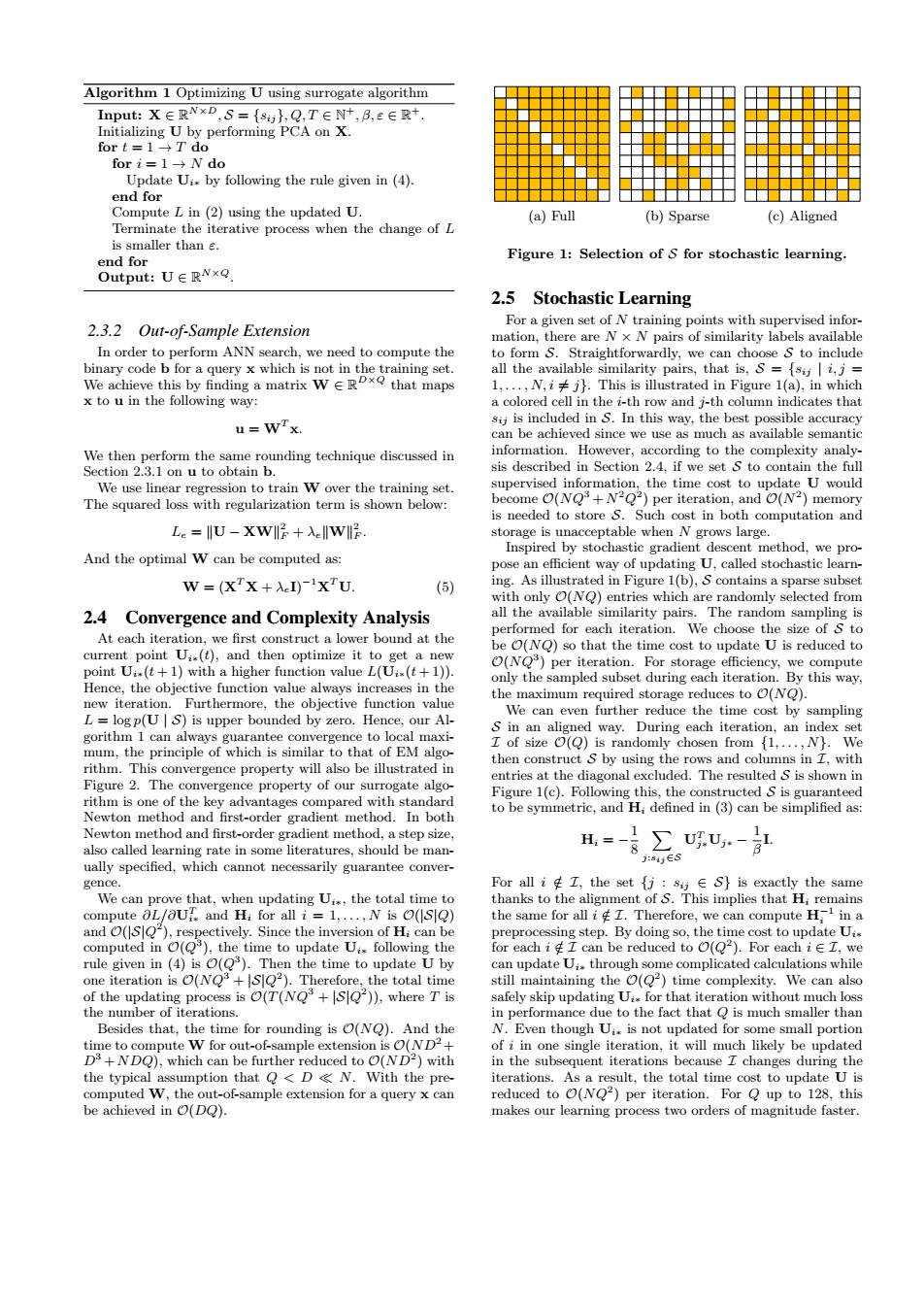And the time to compute W for out-of-sample extension is O(ND2+ D 3 +NDQ), which can be further reduced to O(ND2 ) with the typical assumption that Q < D  N. With the pre￾computed W, the out-of-sample extension for a query x can be achieved in O(DQ). (a) Full (b) Sparse (c) Aligned Figure 1: Selection of S for stochastic learning. 2.5 Stochastic Learning For a given set of N training points with supervised infor￾mation, there are N × N pairs of similarity labels available to form S. Straightforwardly, we can choose S to include all the available similarity pairs, that is, S = {sij | i, j = 1, . . . , N, i 6= j}. This is illustrated in Figure 1(a), in which a colored cell in the i-th row and j-th column indicates that sij is included in S. In this way, the best possible accuracy can be achieved since we use as much as available semantic information. However, according to the complexity analy￾sis described in Section 2.4, if we set S to contain the full supervised information, the time cost to update U would become O(NQ3 + N 2Q 2 ) per iteration, and O(N 2 ) memory is needed to store S. Such cost in both computation and storage is unacceptable when N grows large. Inspired by stochastic gradient descent method, we pro￾pose an efficient way of updating U, called stochastic learn￾ing. As illustrated in Figure 1(b), S contains a sparse subset with only O(NQ) entries which are randomly selected from all the available similarity pairs. The random sampling is performed for each iteration. We choose the size of S to be O(NQ) so that the time cost to update U is reduced to O(NQ3 ) per iteration. For storage efficiency, we compute only the sampled subset during each iteration. By this way, the maximum required storage reduces to O(NQ). We can even further reduce the time cost by sampling S in an aligned way. During each iteration, an index set I of size O(Q) is randomly chosen from {1, . . . , N}. We then construct S by using the rows and columns in I, with entries at the diagonal excluded. The resulted S is shown in Figure 1(c). Following this, the constructed S is guaranteed to be symmetric, and Hi defined in (3) can be simplified as: Hi = − 1 8 X j:sij∈S U T j∗Uj∗ − 1 β I. For all i /∈ I, the set {j : sij ∈ S} is exactly the same thanks to the alignment of S. This implies that Hi remains the same for all i /∈ I. Therefore, we can compute H−1 i in a preprocessing step. By doing so, the time cost to update Ui∗ for each i /∈ I can be reduced to O(Q 2 ). For each i ∈ I, we can update Ui∗ through some complicated calculations while still maintaining the O(Q 2 ) time complexity. We can also safely skip updating Ui∗ for that iteration without much loss in performance due to the fact that Q is much smaller than N. Even though Ui∗ is not updated for some small portion of i in one single iteration, it will much likely be updated in the subsequent iterations because I changes during the iterations. As a result, the total time cost to update U is reduced to O(NQ2 ) per iteration. For Q up to 128, this makes our learning process two orders of magnitude faster