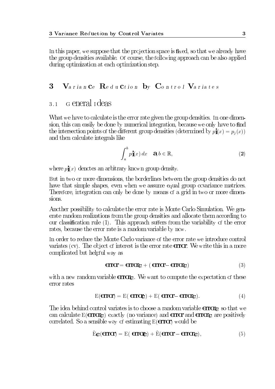
3 Variance Reduction by Control Variates 3 In this paper,we suppose that the prcjection space is fixed,so that we already have the group densities available Of couse,the follcwing approach can be also applied during optimization at each optimization step. 3 Varian Ce Red u Ction by Control variates 3.1 G eneral Ideas What we have to calculate is the error rate given the group densities.In one dimen- sion,this can easily be done by numerical integration,because we only have to find the intersection points of the different group densities(determined by pi)=pi()) and then calculate integrals like pix)dab∈R, (2) where pi)denctes an arbitrary kncwn group density. But in two or more dimensions,the border lines between the group densities do not have that simple shapes,even when we assume equal group ccvariance matrices. Therefore,integration can only be done by means cf a grid in two or more dimen- sions. Ancther possibility to calculate the error rate is Monte Carlo Simulation.We gen- erate random realizations from the group densities and allocate them according to our classification rule (1).This approach suffers from the variability of the error rates,because the error rate is a random variable by ncw. In order to reduce the Monte Carlo variance of the error rate we introduce control variates (cv).The okject cf interest is the error rate errcr.We write this in a more complicated but helpful way as errar=erra+(erra-erra) (3) with a new random variable erra.We want to compute the expectation cf these error rates E(erra)=E(err)+E(rra-erra). (4) The idea behind control variates is to choose a random variable erra so that we can calculate E(erra)exactly (no variance)and error and errorG are positively correlated.So a sensible way cf estimating E(errcr)would be EG(erra)=E(Err)+E(rrar-erra) (5)3 Variance Reduction by Control Variates 3 In this paper, we suppose that the pro jection space is xed, so that we already have the group densities available. Of course, the following approach can be also applied during optimization at each optimization step. 3 Variance Reduction by Control Variates 3.1 General Ideas What we have to calculate is the error rate given the group densities. In one dimen￾sion, this can easily be done by numerical integration, because we only have to nd the intersection points of the dierent group densities (determined by pi(x) = pj (x)) and then calculate integrals like Z b a pi(x) dx a; b 2 R; (2) where pi(x) denotes an arbitrary known group density. But in two or more dimensions, the borderlines between the group densities do not have that simple shapes, even when we assume equal group covariance matrices. Therefore, integration can only be done by means of a grid in two or more dimen￾sions. Another possibility to calculate the error rate is Monte Carlo Simulation. We gen￾erate random realizations from the group densities and allocate them according to our classication rule (1). This approach suers from the variability of the error rates, because the error rate is a random variable by now. In order to reduce the Monte Carlo variance of the error rate we introduce control variates (cv). The ob ject of interest is the error rate error. We write this in a more complicated but helpful way as error = errorcv + ( error￾ errorcv) (3) with a new random variable errorcv . We want to compute the expectation of these error rates E(error) = E( errorcv) + E( error￾ errorcv): (4) The idea behind control variates is to choose a random variable errorcv so that we can calculate E(errorcv) exactly (no variance) and error and errorcv are positively correlated. So a sensible way of estimating E(error) would be E^ cv(error) = E( errorcv) + E( ^ error ￾ errorcv); (5)