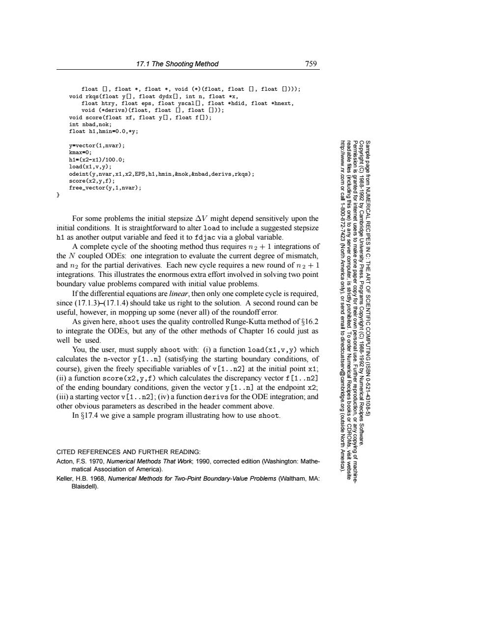
17.1 The Shooting Method 759 float []float *float *void (*)(float,float []float []))) void rkgs(float y[],float dydx],int n,float *x, float htry,float eps,float yscal[],float *hdid,float *hnext, void(*derivs)(f1oat,f1oat[],f1oat☐))： void score(float xf,float y[],float f[]); int nbad,nok; float h1,hmin=0.0,*y; y=vector(1,nvar); kmax=0; h1=(x2-x1)/100.0: load(x1,v,y); odeint(y,nvar,x1,x2,EPS,h1,hmin,&nok,&nbad,derivs,rkqs); score(x2,y,f); free_vector(y,1,nvar); 83g granted for 19881992 11800 For some problems the initial stepsize AV might depend sensitively upon the initial conditions.It is straightforward to alter load to include a suggested stepsize from NUMERICAL RECIPESI h1 as another output variable and feed it to fdjac via a global variable. A complete cycle of the shooting method thus requires n2+1 integrations of the N coupled ODEs:one integration to evaluate the current degree of mismatch, and n2 for the partial derivatives.Each new cycle requires a new round of n2+1 integrations.This illustrates the enormous extra effort involved in solving two point 2a分旧 America computer, boundary value problems compared with initial value problems. If the differential equations are linear,then only one complete cycle is required, since (17.1.3)(17.1.4)should take us right to the solution.A second round can be useful,however,in mopping up some(never all)of the roundoff error. As given here,shoot uses the quality controlled Runge-Kutta method of 816.2 OF SCIENTIFIC to integrate the ODEs,but any of the other methods of Chapter 16 could just as well be used. You,the user,must supply shoot with:(i)a function load(x1,v,y)which calculates the n-vector y[1..n](satisfying the starting boundary conditions,of course),given the freely specifiable variables of v[1..n2]at the initial point x1; (ii)a function score(x2,y,f)which calculates the discrepancy vector f [1..n2] of the ending boundary conditions,given the vector y[1..n]at the endpoint x2: 10621 (iii)a starting vector v[1..n2];(iv)a function derivs for the ODE integration;and other obvious parameters as described in the header comment above. Fuunrggoirioh Numerical Recipes 43106 In $17.4 we give a sample program illustrating how to use shoot. (outside Software. CITED REFERENCES AND FURTHER READING: Ame ying of Acton,F.S.1970,Numerica/Methods That Work;1990,corrected edition (Washington:Mathe- matical Association of America). Keller,H.B.1968,Numerical Methods for Two-Point Boundary-Value Problems (Waltham,MA: Blaisdell).17.1 The Shooting Method 759 Permission is granted for internet users to make one paper copy for their own personal use. Further reproduction, or any copyin Copyright (C) 1988-1992 by Cambridge University Press. Programs Copyright (C) 1988-1992 by Numerical Recipes Software. Sample page from NUMERICAL RECIPES IN C: THE ART OF SCIENTIFIC COMPUTING (ISBN 0-521-43108-5) g of machine￾readable files (including this one) to any server computer, is strictly prohibited. To order Numerical Recipes books or CDROMs, visit website http://www.nr.com or call 1-800-872-7423 (North America only), or send email to directcustserv@cambridge.org (outside North America). float [], float *, float *, void (*)(float, float [], float []))); void rkqs(float y[], float dydx[], int n, float *x, float htry, float eps, float yscal[], float *hdid, float *hnext, void (*derivs)(float, float [], float [])); void score(float xf, float y[], float f[]); int nbad,nok; float h1,hmin=0.0,*y; y=vector(1,nvar); kmax=0; h1=(x2-x1)/100.0; load(x1,v,y); odeint(y,nvar,x1,x2,EPS,h1,hmin,&nok,&nbad,derivs,rkqs); score(x2,y,f); free_vector(y,1,nvar); } For some problems the initial stepsize ∆V might depend sensitively upon the initial conditions. It is straightforward to alter load to include a suggested stepsize h1 as another output variable and feed it to fdjac via a global variable. A complete cycle of the shooting method thus requires n2 + 1 integrations of the N coupled ODEs: one integration to evaluate the current degree of mismatch, and n2 for the partial derivatives. Each new cycle requires a new round of n 2 + 1 integrations. This illustrates the enormous extra effort involved in solving two point boundary value problems compared with initial value problems. If the differential equations are linear, then only one complete cycle is required, since (17.1.3)–(17.1.4) should take us right to the solution. A second round can be useful, however, in mopping up some (never all) of the roundoff error. As given here, shoot uses the quality controlled Runge-Kutta method of §16.2 to integrate the ODEs, but any of the other methods of Chapter 16 could just as well be used. You, the user, must supply shoot with: (i) a function load(x1,v,y) which calculates the n-vector y[1..n] (satisfying the starting boundary conditions, of course), given the freely specifiable variables of v[1..n2] at the initial point x1; (ii) a function score(x2,y,f) which calculates the discrepancy vector f[1..n2] of the ending boundary conditions, given the vector y[1..n] at the endpoint x2; (iii) a starting vector v[1..n2]; (iv) a function derivs for the ODE integration; and other obvious parameters as described in the header comment above. In §17.4 we give a sample program illustrating how to use shoot. CITED REFERENCES AND FURTHER READING: Acton, F.S. 1970, Numerical Methods That Work; 1990, corrected edition (Washington: Mathe￾matical Association of America). Keller, H.B. 1968, Numerical Methods for Two-Point Boundary-Value Problems (Waltham, MA: Blaisdell)