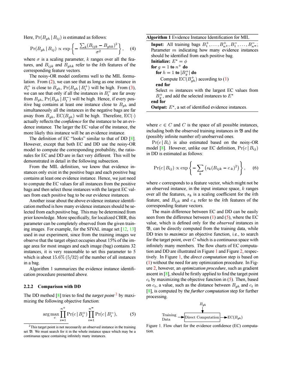
Here,Pr(Bah Bij)is estimated as follows: Algorithm 1 Evidence Instance Identification for MIL Input:All training bags B,....B+,Br,....B-; Pr(Bgh Bij)exp ∫_∑A(Bk-Bghk2 Parameter m indicating how many evidence instances should be identified from each positive bag. where o is a scaling parameter,k ranges over all the fea- Initialize:E*=中 tures,and Bijk and Bahk refer to the kth features of the corresponding feature vectors. for g =1 to n+do for h 1 to B do The noisy-OR model conforms well to the MIL formu- lation.From(2),we can see that as long as one instance in Compute EC(B)according to (1) end for B is close to Bah,Pr(Bgh B)will be high.From (3), we can see that only if all the instances in B are far away Select m instances with the largest EC values from from Boh,Pr(Bgh B)will be high.Hence,if every pos- B,and add the selected instances to E* end for itive bag contains at least one instance close to Bgh and simultaneously all the instances in the negative bags are far Output:E*,a set of identified evidence instances away from Boh,EC(Bah)will be high.Therefore,EC() actually reflects the confidence for the instance to be an evi- dence instance.The larger the EC value of the instance,the where c E C and C is the space of all possible instances, more likely this instance will be an evidence instance. including both the observed training instances in B and the The definition of EC "looks"similar to that of DD [8]. (possibly infinite number of)unobserved ones. However,except that both EC and DD use the noisy-OR Pr(c|B:)is also estimated based on the noisy-OR model to compute the corresponding probability,the ratio- model [8].However,unlike our EC definition,Pr(c Bij) nales for EC and DD are in fact very different.This will be in DD is estimated as follows: demonstrated in detail in the following subsection. From the MIL definition.we know that evidence in- Pr(c|B）o stances only exist in the positive bags and each positive bag -∑Bk- (6) contains at least one evidence instance.Hence,we just need to compute the EC values for all instances from the positive where c corresponds to a feature vector,which might not be bags and then select those instances with the largest EC val- an observed instance,in the input instance space,k ranges ues from each positive bag to be our evidence instances. over all the features,s is a scaling coefficient for the kth Another issue about the above evidence instance identifi- feature,and Bijk and c.refer to the kth features of the cation method is how many evidence instances should be se- corresponding feature vectors. lected from each positive bag.This may be determined from The main difference between EC and DD can be easily prior knowledge.More specifically,for localized CBIR,this seen from the difference between(1)and(5),where the EC parameter can be completely observed from the given train- value,which is defined only for the observed instances in ing images.For example,for the SIVAL image set [12,13] B,can be directly computed from the training data,while used in our experiment,since from the training images we DD tries to maximize an objective function,i.e..to search observe that the target object occupies about 15%of the im- for the target point,over C which is a continuous space with age area for most images and each image(bag)contains 32 infinitely many members.The flow charts of EC computa- instances,it is very reasonable to set this parameter to 5 tion and DD are illustrated in Figure I and Figure 2.respec- which is about 15.6%(5/32)of the number of all instances tively.In Figure 1,the direct computation step is based on in a bag (1)without the need for any optimization procedure.In Fig- Algorithm 1 summarizes the evidence instance identifi- ure 2,however,an optimization procedure,such as gradient cation procedure presented above. ascent in [8],should be firstly applied to find the target point ct by maximizing the objective function in (5).Then,based 2.2.2 Comparison with DD on ct,a value,such as the distance between Bah and c in [8],is computed by the further computation step for further The DD method [8]tries to find the target point2 by maxi- processing. mizing the following objective function: arg may (c B cB), 5 Training Data Direct Computation +EC(Bgh) 2This target point is not necessarily an observed instance in the training Figure 1.Flow chart for the evidence confidence (EC)computa- set B.We must search for it in the whole instance space which may be a tion. continuous space containing infinitely many instances.Here, Pr(Bgh | Bij ) is estimated as follows: Pr(Bgh | Bij ) ∝ exp  − P k (Bijk − Bghk) 2 σ 2  , (4) where σ is a scaling parameter, k ranges over all the fea￾tures, and Bijk and Bghk refer to the kth features of the corresponding feature vectors. The noisy-OR model conforms well to the MIL formu￾lation. From (2), we can see that as long as one instance in B + i is close to Bgh, Pr(Bgh | B + i ) will be high. From (3), we can see that only if all the instances in B − i are far away from Bgh, Pr(Bgh | B − i ) will be high. Hence, if every pos￾itive bag contains at least one instance close to Bgh and simultaneously all the instances in the negative bags are far away from Bgh, EC(Bgh) will be high. Therefore, EC(·) actually reflects the confidence for the instance to be an evi￾dence instance. The larger the EC value of the instance, the more likely this instance will be an evidence instance. The definition of EC “looks” similar to that of DD [8]. However, except that both EC and DD use the noisy-OR model to compute the corresponding probability, the ratio￾nales for EC and DD are in fact very different. This will be demonstrated in detail in the following subsection. From the MIL definition, we know that evidence in￾stances only exist in the positive bags and each positive bag contains at least one evidence instance. Hence, we just need to compute the EC values for all instances from the positive bags and then select those instances with the largest EC val￾ues from each positive bag to be our evidence instances. Another issue about the above evidence instance identifi- cation method is how many evidence instances should be se￾lected from each positive bag. This may be determined from prior knowledge. More specifically, for localized CBIR, this parameter can be completely observed from the given train￾ing images. For example, for the SIVAL image set [12, 13] used in our experiment, since from the training images we observe that the target object occupies about 15% of the im￾age area for most images and each image (bag) contains 32 instances, it is very reasonable to set this parameter to 5 which is about 15.6% (5/32) of the number of all instances in a bag. Algorithm 1 summarizes the evidence instance identifi- cation procedure presented above. 2.2.2 Comparison with DD The DD method [8] tries to find the target point 2 by maxi￾mizing the following objective function: arg max c nY+ i=1 Pr(c | B + i ) nY− i=1 Pr(c | B − i ), (5) 2This target point is not necessarily an observed instance in the training set B. We must search for it in the whole instance space which may be a continuous space containing infinitely many instances. Algorithm 1 Evidence Instance Identification for MIL Input: All training bags B + 1 , . . . , B+ n+ , B− 1 , . . . , B− n− ; Parameter m indicating how many evidence instances should be identified from each positive bag. Initialize: E∗ = φ for g = 1 to n + do for h = 1 to |B+ g | do Compute EC(B + gh) according to (1) end for Select m instances with the largest EC values from B+ g , and add the selected instances to E∗ end for Output: E∗ , a set of identified evidence instances. where c ∈ C and C is the space of all possible instances, including both the observed training instances in B and the (possibly infinite number of) unobserved ones. Pr(c | Bi) is also estimated based on the noisy-OR model [8]. However, unlike our EC definition, Pr(c | Bij ) in DD is estimated as follows: Pr(c | Bij ) ∝ exp ( − X k ￾ sk(Bijk − c·k) 2
) , (6) where c corresponds to a feature vector, which might not be an observed instance, in the input instance space, k ranges over all the features, sk is a scaling coefficient for the kth feature, and Bijk and c·k refer to the kth features of the corresponding feature vectors. The main difference between EC and DD can be easily seen from the difference between (1) and (5), where the EC value, which is defined only for the observed instances in B, can be directly computed from the training data, while DD tries to maximize an objective function, i.e., to search for the target point, over C which is a continuous space with infinitely many members. The flow charts of EC computa￾tion and DD are illustrated in Figure 1 and Figure 2, respec￾tively. In Figure 1, the direct computation step is based on (1) without the need for any optimization procedure. In Fig￾ure 2, however, an optimization procedure, such as gradient ascent in [8], should be firstly applied to find the target point ct by maximizing the objective function in (5). Then, based on ct, a value, such as the distance between Bgh and ct in [8], is computed by the further computation step for further processing. Training Data Bgh Direct Computation EC(Bgh) Figure 1. Flow chart for the evidence confidence (EC) computa￾tion