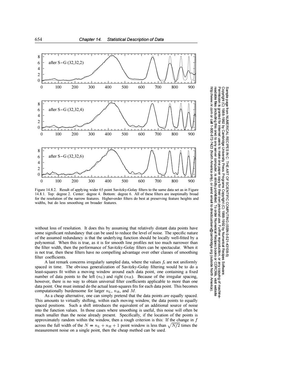
654 Chapter 14.Statistical Description of Data 6 after S-G(32.32.2) 2 0 0 100 200 300 400500600 700800 900 after S-G(32.32,4) E 83g 23 granted for 19881992 0 1-.200 0 100 200 300 400500 600 700 800 900 from NUMERICAL RECIPESI 8TT+T++T 6 after S-G(32.32,6) server (Nor to make 4 America computer, THE mw,,1,,,,1,,,,1, ART 0 100.200300400500600700800 900 9 Programs Figure 14.8.2.Result of applying wider 65 point Savitzky-Golay filters to the same data set as in Figure 14.8.1.Top:degree 2.Center:degree 4.Bottom:degree 6.All of these filters are inoptimally broad for the resolution of the narrow features.Higher-order filters do best at preserving feature heights and widths,but do less smoothing on broader features. 兰云侯 to dir OF SCIENTIFIC COMPUTING(ISBN without loss of resolution.It does this by assuming that relatively distant data points have 1988-19920 some significant redundancy that can be used to reduce the level of noise.The specific nature of the assumed redundancy is that the underlying function should be locally well-fitted by a 10-621 polynomial.When this is true,as it is for smooth line profiles not too much narrower than the filter width,then the performance of Savitzky-Golay filters can be spectacular.When it idge.org Numerical Recipes 43108 is not true,then these filters have no compelling advantage over other classes of smoothing filter coefficients. A last remark concerns irregularly sampled data,where the values fi are not uniformly (outside spaced in time.The obvious generalization of Savitzky-Golay filtering would be to do a least-squares fit within a moving window around each data point,one containing a fixed North Software. number of data points to the left (nL)and right(nR).Because of the irregular spacing. however,there is no way to obtain universal filter coefficients applicable to more than one data point.One must instead do the actual least-squares fits for each data point.This becomes computationally burdensome for larger nL,nR,and M. As a cheap alternative,one can simply pretend that the data points are equally spaced. This amounts to virtually shifting,within each moving window,the data points to equally spaced positions.Such a shift introduces the equivalent of an additional source of noise into the function values.In those cases where smoothing is useful,this noise will often be much smaller than the noise already present.Specifically,if the location of the points is approximately random within the window,then a rough criterion is this:If the change in f across the full width of the N =nL+nR+1 point window is less than VN/2 times the measurement noise on a single point,then the cheap method can be used.654 Chapter 14. Statistical Description of Data Permission is granted for internet users to make one paper copy for their own personal use. Further reproduction, or any copyin Copyright (C) 1988-1992 by Cambridge University Press. Programs Copyright (C) 1988-1992 by Numerical Recipes Software. Sample page from NUMERICAL RECIPES IN C: THE ART OF SCIENTIFIC COMPUTING (ISBN 0-521-43108-5) g of machine￾readable files (including this one) to any server computer, is strictly prohibited. To order Numerical Recipes books or CDROMs, visit website http://www.nr.com or call 1-800-872-7423 (North America only), or send email to directcustserv@cambridge.org (outside North America). after S–G (32,32,4) after S–G (32,32,2) 8 6 4 2 0 0 100 200 300 400 500 600 700 800 900 8 6 4 2 0 after S–G (32,32,6) 0 100 200 300 400 500 600 700 800 900 8 6 4 2 0 0 100 200 300 400 500 600 700 800 900 Figure 14.8.2. Result of applying wider 65 point Savitzky-Golay filters to the same data set as in Figure 14.8.1. Top: degree 2. Center: degree 4. Bottom: degree 6. All of these filters are inoptimally broad for the resolution of the narrow features. Higher-order filters do best at preserving feature heights and widths, but do less smoothing on broader features. without loss of resolution. It does this by assuming that relatively distant data points have some significant redundancy that can be used to reduce the level of noise. The specific nature of the assumed redundancy is that the underlying function should be locally well-fitted by a polynomial. When this is true, as it is for smooth line profiles not too much narrower than the filter width, then the performance of Savitzky-Golay filters can be spectacular. When it is not true, then these filters have no compelling advantage over other classes of smoothing filter coefficients. A last remark concerns irregularly sampled data, where the values fi are not uniformly spaced in time. The obvious generalization of Savitzky-Golay filtering would be to do a least-squares fit within a moving window around each data point, one containing a fixed number of data points to the left (nL) and right (nR). Because of the irregular spacing, however, there is no way to obtain universal filter coefficients applicable to more than one data point. One must instead do the actual least-squares fits for each data point. This becomes computationally burdensome for larger nL, nR, and M. As a cheap alternative, one can simply pretend that the data points are equally spaced. This amounts to virtually shifting, within each moving window, the data points to equally spaced positions. Such a shift introduces the equivalent of an additional source of noise into the function values. In those cases where smoothing is useful, this noise will often be much smaller than the noise already present. Specifically, if the location of the points is approximately random within the window, then a rough criterion is this: If the change in f across the full width of the N = nL + nR + 1 point window is less than N/2 times the measurement noise on a single point, then the cheap method can be used