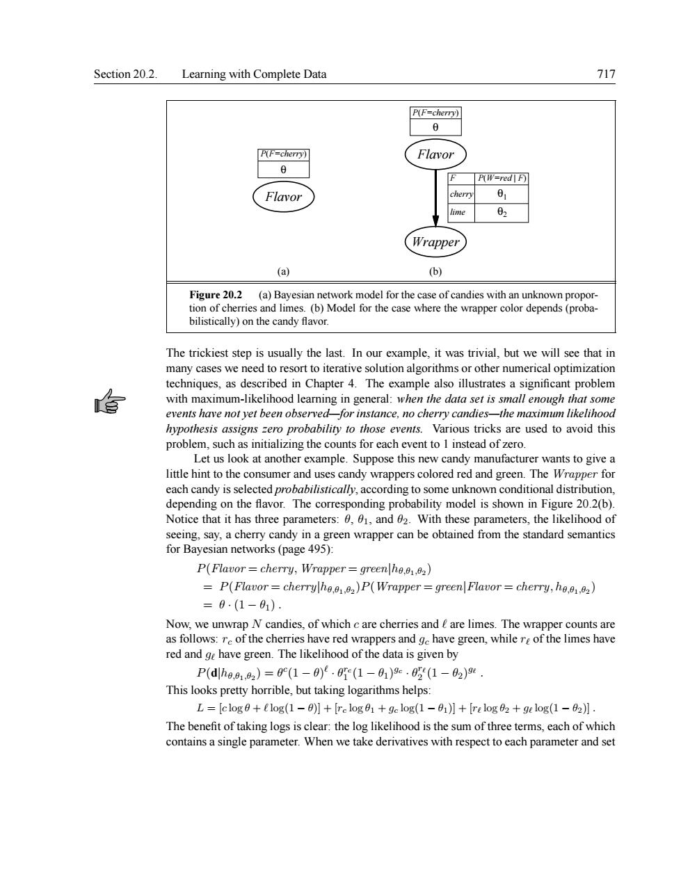
Section 20.2.Learning with Complete Data 717 PF-cherry】 PF-chery) Flavor ☐PW=ed Flavor Wrapper (a ) bilistically)on the candy flavor. The trickiest step is usually the last.In our example,it was trivial,but we will see that in eed to ort to iterative solution algorithn encaloptimizaion oblen ood eari eral n the datd set is s et be a ricks are used to avoid this ing the cou or each event to1 insteado uppose th wants to give The W. for eachcandy es candy wrappers orodedandgre is sele ilistically, s,the 4e20 thre arameters param eliho ined from the standard semantics P(Flavor=cherry,Wrapper=greenho.0.0) =P(Flavor= cherrylho)P(Wrapper=green Flavor=cherry,ho.0.) =0.1-01) 网a阿 P(dhe.a1,2）=0r(1-0.(1-a)e.(1-a2)9 This looks pretty horrible,but taking logarithms help L [clog0+6l0g(1-0)]+[re log01+ge log(1-01)]+[relog 02 ge log(1-02)]. The benefit of taking logs is clear:the log likelihood is the sum of three terms each of which contains a single parameter.When we take derivatives with respect to each parameter and setSection 20.2. Learning with Complete Data 717 Flavor P(F=cherry) (a) θ P(F=cherry) Flavor Wrapper (b) θ F cherry lime P(W=red | F) θ1 θ2 Figure 20.2 (a) Bayesian network model for the case of candies with an unknown propor￾tion of cherries and limes. (b) Model for the case where the wrapper color depends (proba￾bilistically) on the candy flavor. The trickiest step is usually the last. In our example, it was trivial, but we will see that in many cases we need to resort to iterative solution algorithms or other numerical optimization techniques, as described in Chapter 4. The example also illustrates a significant problem with maximum-likelihood learning in general: when the data set is small enough that some events have not yet been observed—for instance, no cherry candies—the maximum likelihood hypothesis assigns zero probability to those events. Various tricks are used to avoid this problem, such as initializing the counts for each event to 1 instead of zero. Let us look at another example. Suppose this new candy manufacturer wants to give a little hint to the consumer and uses candy wrappers colored red and green. The Wrapper for each candy is selected probabilistically, according to some unknown conditional distribution, depending on the flavor. The corresponding probability model is shown in Figure 20.2(b). Notice that it has three parameters: θ, θ1, and θ2. With these parameters, the likelihood of seeing, say, a cherry candy in a green wrapper can be obtained from the standard semantics for Bayesian networks (page 495): P(Flavor = cherry,Wrapper = green|hθ,θ1,θ2 ) = P(Flavor = cherry|hθ,θ1,θ2 )P(Wrapper = green|Flavor = cherry, hθ,θ1,θ2 ) = θ · (1 − θ1) . Now, we unwrap N candies, of which c are cherries and ` are limes. The wrapper counts are as follows: rc of the cherries have red wrappers and gc have green, while r` of the limes have red and g` have green. The likelihood of the data is given by P(d|hθ,θ1,θ2 ) = θ c (1 − θ) ` · θ rc 1 (1 − θ1) gc · θ r` 2 (1 − θ2) g` . This looks pretty horrible, but taking logarithms helps: L = [c log θ + ` log(1 − θ)] + [rc log θ1 + gc log(1 − θ1)] + [r` log θ2 + g` log(1 − θ2)] . The benefit of taking logs is clear: the log likelihood is the sum of three terms, each of which contains a single parameter. When we take derivatives with respect to each parameter and set