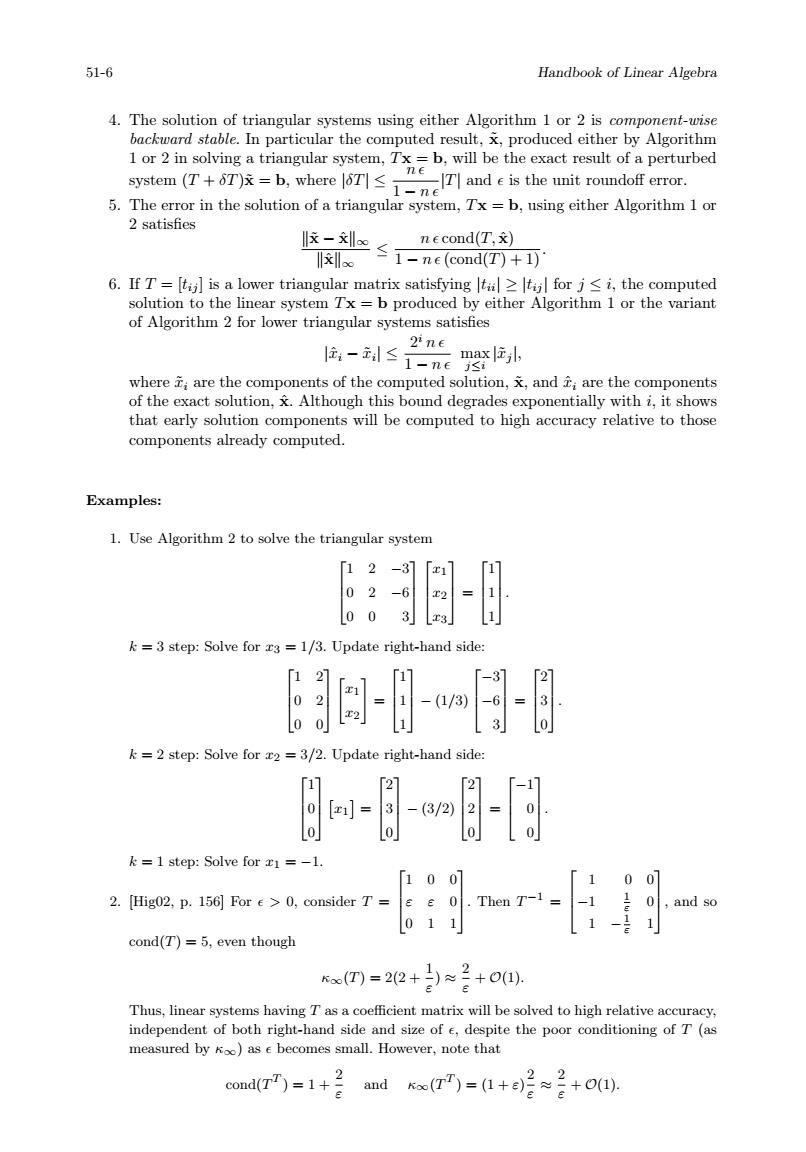
51-6 Handbook of Linear Algebra Algorithm 1 or 2 is 102 rith solvin r sy system (T+6T)=b,where |6T]< -T and e is the unit roundoff error. 2 satisfios necond(T.) x 6.If T=[t]is a lower triangular matrix satisfying for jsi,the co solution to the line of Algorithm 2 for lower triangular systems satisfies -≤ where are the of the exact solution,Although this bound degrades onentially with i,it sho that early solution components will be computed to high accuracy relative to those components already computed. Examples: 1.Use Algorithm 2 to solve the triangular system k=3 step:Solve for r3=1/3.Update right-hand side 阳-月日月 =2 step:Solve for2=3/2.Update right-hand sides =1 step:Solve for=- 100 2.[Hig02,p.156]For e>0,consider T= cond(T)=5,even though x(四)=22+3≈2+0. Thus,lin ms having T as a coefficient matrix will be solved to high relative ent of both right-hand side and size of des te the poor conditioning of T(as small.However,note that cond(TT)=1+2 and (TT)=(1+e)22+(1).51-6 Handbook of Linear Algebra 4. The solution of triangular systems using either Algorithm 1 or 2 is component-wise backward stable. In particular the computed result, x˜, produced either by Algorithm 1 or 2 in solving a triangular system, Tx = b, will be the exact result of a perturbed system (T + δT)x˜ = b, where |δT| ≤ n  1 − n  |T| and  is the unit roundoff error. 5. The error in the solution of a triangular system, Tx = b, using either Algorithm 1 or 2 satisfies kx˜ − xˆk∞ kxˆk∞ ≤ n  cond(T, xˆ) 1 − n  (cond(T) + 1). 6. If T = [tij ] is a lower triangular matrix satisfying |tii| ≥ |tij | for j ≤ i, the computed solution to the linear system Tx = b produced by either Algorithm 1 or the variant of Algorithm 2 for lower triangular systems satisfies |xˆi − x˜i | ≤ 2 i n  1 − n  max j≤i |x˜j |, where ˜xi are the components of the computed solution, x˜, and ˆxi are the components of the exact solution, xˆ. Although this bound degrades exponentially with i, it shows that early solution components will be computed to high accuracy relative to those components already computed. Examples: 1. Use Algorithm 2 to solve the triangular system    1 2 −3 0 2 −6 0 0 3       x1 x2 x3    =    1 1 1   . k = 3 step: Solve for x3 = 1/3. Update right-hand side:    1 2 0 2 0 0    " x1 x2 # =    1 1 1    − (1/3)    −3 −6 3    =    2 3 0   . k = 2 step: Solve for x2 = 3/2. Update right-hand side:    1 0 0    x1 =    2 3 0    − (3/2)    2 2 0    =    −1 0 0   . k = 1 step: Solve for x1 = −1. 2. [Hig02, p. 156] For  > 0, consider T =    1 0 0 ε ε 0 0 1 1    . Then T −1 =    1 0 0 −1 1 ε 0 1 − 1 ε 1   , and so cond(T) = 5, even though κ∞(T) = 2(2 + 1 ε ) ≈ 2 ε + O(1). Thus, linear systems having T as a coefficient matrix will be solved to high relative accuracy, independent of both right-hand side and size of , despite the poor conditioning of T (as measured by κ∞) as  becomes small. However, note that cond(T T ) = 1 + 2 ε and κ∞(T T ) = (1 + ε) 2 ε ≈ 2 ε + O(1).