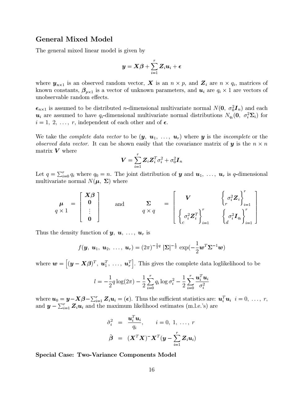
General Mixed Model The general mixed linear model is given by y=XB+∑Z:u:+e =1 where ynxi is an observed random vector,X is an n x p,and Zi are n x gi,matrices of known constants,Bpxi is a vector of unknown parameters,and ui are qax 1 are vectors of unobservable random effects. enxi1 is assumed to be distributed n-dimensional multivariate normal N(0,oIn)and each ui are assumed to have qi-dimensional multivariate normal distributions Na(0,oi)for i=1,2,...r,independent of each other and of e. We take the complete data vector to be (y,u1,...,ur)where y is the incomplete or the observed data vector.It can be shown easily that the covariance matrix of y is the n x n matrix V where V=∑Z:Zo+oIn i=1 Let where go=n.The joint distribution of y and ui,...,ur is g-dimensional multivariate normal N(u,>)where 「 XB 0 and 9×1 0 Thus the density function of y,u,...,ur is ...(2xpww) where w=(y-XB)T,uf,...,uT.This gives the complete data loglikelihood to be 1=-log2）- 1 一。ogo是2>6 =0 where uo=y-XB-Ziui=(e).Thus the sufficient statistics are:uuii=0,...,r, and y-Ziu;and the maximum likelihood estimates (m.l.e.'s)are i=0,1,..,r 3=(XTX)XT(y-∑Z:u) i=1 Special Case:Two-Variance Components Model 16General Mixed Model The general mixed linear model is given by y = Xβ + Xr i=1 Ziui +  where yn×1 is an observed random vector, X is an n × p, and Zi are n × qi , matrices of known constants, βp×1 is a vector of unknown parameters, and ui are qi × 1 are vectors of unobservable random effects. n×1 is assumed to be distributed n-dimensional multivariate normal N(0, σ 2 0In) and each ui are assumed to have qi-dimensional multivariate normal distributions Nqi (0, σ 2 i Σi) for i = 1, 2, . . . , r, independent of each other and of . We take the complete data vector to be (y, u1, . . . , ur) where y is the incomplete or the observed data vector. It can be shown easily that the covariance matrix of y is the n × n matrix V where V = Xr i=1 ZiZ T i σ 2 i + σ 2 0In Let q = Pr i=0 qi where q0 = n. The joint distribution of y and u1, . . . , ur is q-dimensional multivariate normal N(µ, Σ) where µ = q × 1       Xβ 0 . . . 0       and Σ = q × q        V ( r σ 2 i Zi )r i=1 ( c σ 2 i Z T i )r i=1 ( d σ 2 i Iqi )r i=1        Thus the density function of y, u, . . . , ur is f(y, u1, u2, . . . , ur) = (2π) − 1 2 q |Σ| − 1 2 exp(− 1 2 wT Σ −1w) where w = h (y − Xβ) T , u T 1 , . . . , u T r i . This gives the complete data loglikelihood to be l = − 1 2 q log(2π) − 1 2 Xr i=0 qi log σ 2 i − 1 2 Xr i=0 u T i ui σ 2 i where u0 = y−Xβ− Pr i=1 Ziui = (). Thus the sufficient statistics are: u T i ui i = 0, . . . , r, and y − Pr i=1 Ziui and the maximum likelihood estimates (m.l.e.’s) are σˆ 2 i = u T i ui qi , i = 0, 1, . . . , r βˆ = (XTX) −XT (y − Xr i=1 Ziui) Special Case: Two-Variance Components Model 16