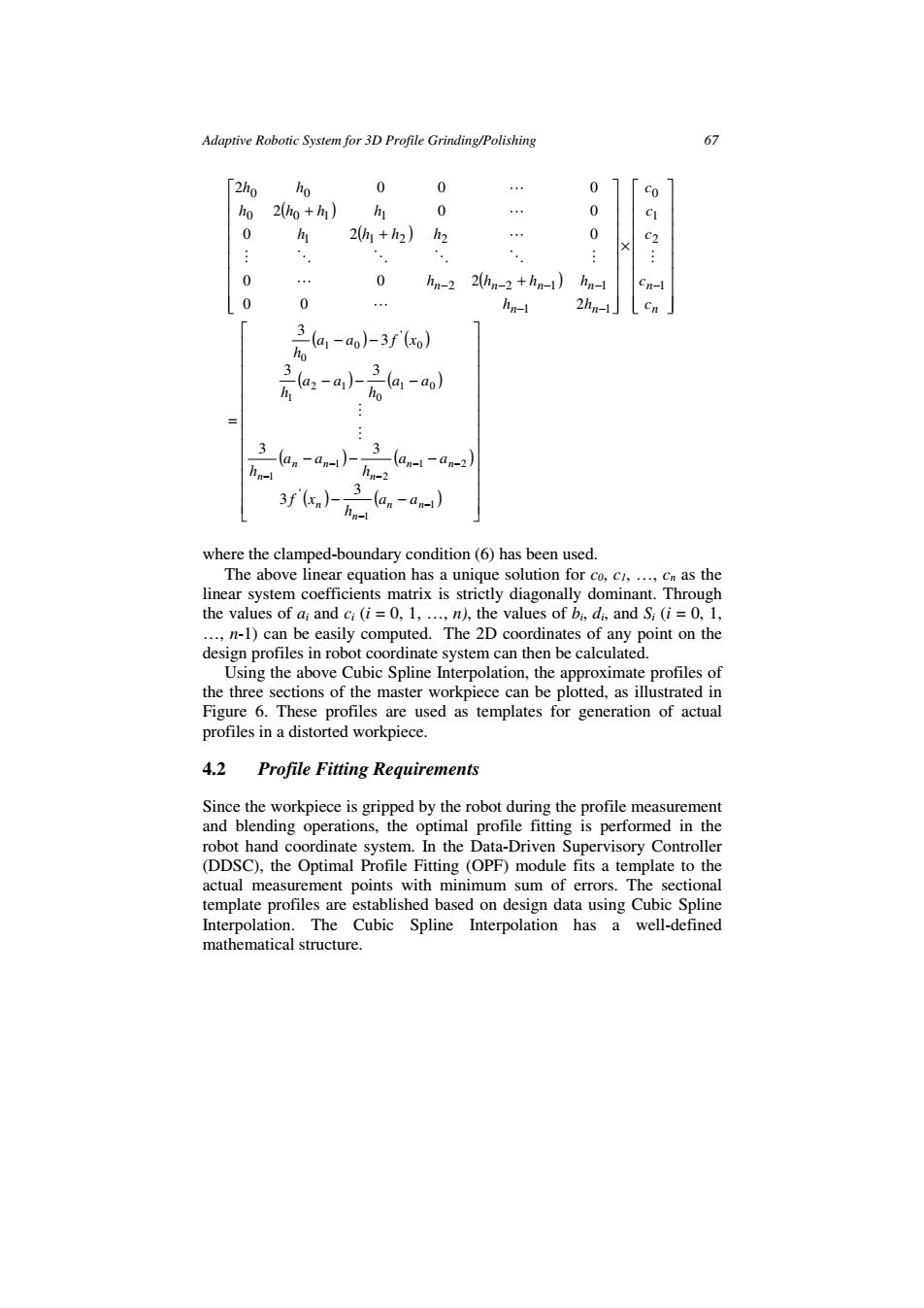
Adaptive Robotic System for 3D Profile Grinding/Polishing 67 2ho ho 0 0 0 Co ho 2(ho+) h 0 0 9 0 h 2h1+h2）h2 0 C2 0 … 0 hn-22hn-2+hn-） hn- Cn-1 0 0 hn-1 2hn-1] Cn 3a,-ao)-3f(o） n一a1)-(a1-a0 h (anan-1)-h 3_an1-am-2 3fx,广ha.-a-） where the clamped-boundary condition(6)has been used. The above linear equation has a unique solution for co,ci,...,c as the linear system coefficients matrix is strictly diagonally dominant.Through the values of a;and ci(i=0,1,...n),the values of bi,di,and Si(i=0,1, ...n-1)can be easily computed.The 2D coordinates of any point on the design profiles in robot coordinate system can then be calculated. Using the above Cubic Spline Interpolation,the approximate profiles of the three sections of the master workpiece can be plotted,as illustrated in Figure 6.These profiles are used as templates for generation of actual profiles in a distorted workpiece. 4.2 Profile Fitting Requirements Since the workpiece is gripped by the robot during the profile measurement and blending operations,the optimal profile fitting is performed in the robot hand coordinate system.In the Data-Driven Supervisory Controller (DDSC),the Optimal Profile Fitting (OPF)module fits a template to the actual measurement points with minimum sum of errors.The sectional template profiles are established based on design data using Cubic Spline Interpolation.The Cubic Spline Interpolation has a well-defined mathematical structure.Adaptive Robotic System for 3D Profile Grinding/Polishing 67 ( ) ( ) ( )                     ×                     + + + − − − − − − − n n n n n n n n c c c c c h h h h h h h h h h h h h h h h 1 2 1 0 1 1 2 2 1 1 1 1 2 2 0 0 1 1 0 0 0 0 2 0 0 2 0 2 0 2 0 0 2 0 0 0 M L L M O O O O M L L L ( ) ( ) ( ) ( ) ( ) ( ) ( ) ( )                             − − − − − − − − − − = − − − − − − − 1 1 ' 1 2 2 1 1 1 0 0 2 1 1 0 ' 1 0 0 3 3 3 3 3 3 3 3 n n n n n n n n n n a a h xf a a h a a h a a h a a h a a xf h M M where the clamped-boundary condition (6) has been used. The above linear equation has a unique solution for c0, c1, …, cn as the linear system coefficients matrix is strictly diagonally dominant. Through the values of ai and ci (i = 0, 1, …, n), the values of bi, di, and Si (i = 0, 1, …, n-1) can be easily computed. The 2D coordinates of any point on the design profiles in robot coordinate system can then be calculated. Using the above Cubic Spline Interpolation, the approximate profiles of the three sections of the master workpiece can be plotted, as illustrated in Figure 6. These profiles are used as templates for generation of actual profiles in a distorted workpiece. 4.2 Profile Fitting Requirements Since the workpiece is gripped by the robot during the profile measurement and blending operations, the optimal profile fitting is performed in the robot hand coordinate system. In the Data-Driven Supervisory Controller (DDSC), the Optimal Profile Fitting (OPF) module fits a template to the actual measurement points with minimum sum of errors. The sectional template profiles are established based on design data using Cubic Spline Interpolation. The Cubic Spline Interpolation has a well-defined mathematical structure