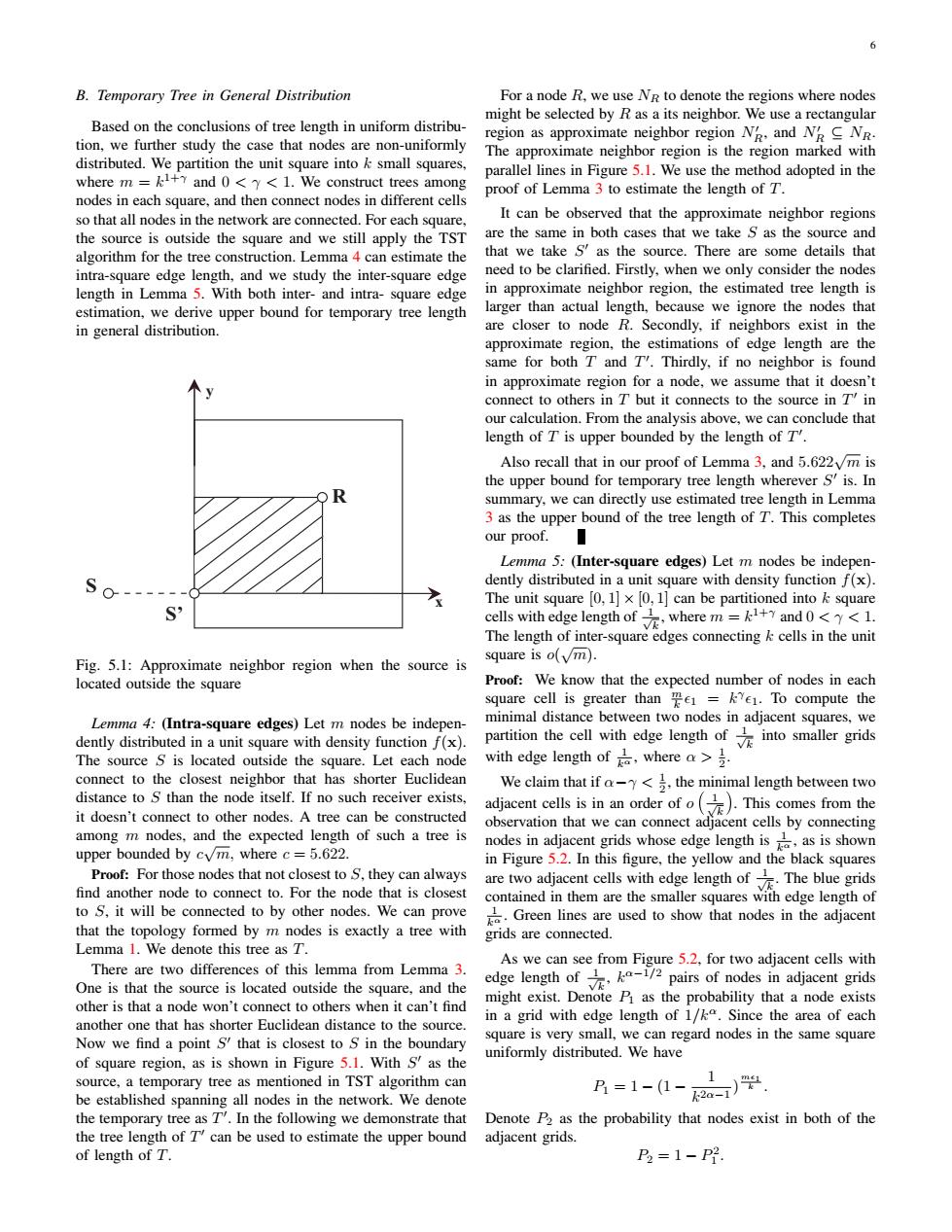
6 B.Temporary Tree in General Distribution For a node R,we use NR to denote the regions where nodes might be selected by R as a its neighbor.We use a rectangular Based on the conclusions of tree length in uniform distribu- region as approximate neighbor region N.and N C NR. tion,we further study the case that nodes are non-uniformly The approximate neighbor region is the region marked with distributed.We partition the unit square into k small squares, where m =k1+7 and 0<Y<1.We construct trees among parallel lines in Figure 5.1.We use the method adopted in the proof of Lemma 3 to estimate the length of T. nodes in each square,and then connect nodes in different cells so that all nodes in the network are connected.For each square, It can be observed that the approximate neighbor regions the source is outside the square and we still apply the TST are the same in both cases that we take S as the source and algorithm for the tree construction.Lemma 4 can estimate the that we take S'as the source.There are some details that intra-square edge length,and we study the inter-square edge need to be clarified.Firstly,when we only consider the nodes length in Lemma 5.With both inter-and intra-square edge in approximate neighbor region,the estimated tree length is estimation,we derive upper bound for temporary tree length larger than actual length,because we ignore the nodes that in general distribution. are closer to node R.Secondly,if neighbors exist in the approximate region,the estimations of edge length are the same for both T and T.Thirdly,if no neighbor is found in approximate region for a node,we assume that it doesn't connect to others in T but it connects to the source in T in our calculation.From the analysis above,we can conclude that length of T is upper bounded by the length of T. Also recall that in our proof of Lemma 3,and 5.622vm is the upper bound for temporary tree length wherever S'is.In summary,we can directly use estimated tree length in Lemma 3 as the upper bound of the tree length of T.This completes our proof. Lemma 5:(Inter-square edges)Let m nodes be indepen- So- dently distributed in a unit square with density function f(x). The unit square [0,1]x [0,1]can be partitioned into k square S, cells with edge length of1 where m=k+and0<<1. The length of inter-square edges connecting k cells in the unit Fig.5.1:Approximate neighbor region when the source is square is o(vm). located outside the square Proof:We know that the expected number of nodes in each square cell is greater than e=kYe1.To compute the Lemma 4:(Intra-square edges)Let m nodes be indepen- minimal distance between two nodes in adjacent squares,we dently distributed in a unit square with density function f(x). partition the cell with edge length ofinto smaller grids The source S is located outside the square.Let each node with edge length of where a>. connect to the closest neighbor that has shorter Euclidean We claim that if a-<,the minimal length between two distance to S than the node itself.If no such receiver exists. adjacent cells is in an order of This comes from the it doesn't connect to other nodes.A tree can be constructed observation that we can connect adjacent cells by connecting among m nodes,and the expected length of such a tree is upper bounded by cvm,where c=5.622. nodes in adjacent grids whose edge length is as is shown in Figure 5.2.In this figure,the yellow and the black squares Proof:For those nodes that not closest to S,they can always are two adjacent cells with edge length of The blue grids find another node to connect to.For the node that is closest contained in them are the smaller squares with edge length of to S,it will be connected to by other nodes.We can prove Green lines are used to show that nodes in the adjacent that the topology formed by m nodes is exactly a tree with grids are connected. Lemma 1.We denote this tree as T. As we can see from Figure 5.2,for two adjacent cells with There are two differences of this lemma from Lemma 3. One is that the source is located outside the square,and the edge length of12 pairs of nodes in adjacent grids might exist.Denote P as the probability that a node exists other is that a node won't connect to others when it can't find another one that has shorter Euclidean distance to the source. in a grid with edge length of 1/k.Since the area of each Now we find a point S'that is closest to S in the boundary square is very small,we can regard nodes in the same square uniformly distributed.We have of square region,as is shown in Figure 5.1.With S as the source,a temporary tree as mentioned in TST algorithm can be established spanning all nodes in the network.We denote A=1-1-学 the temporary tree as T.In the following we demonstrate that Denote P2 as the probability that nodes exist in both of the the tree length of T can be used to estimate the upper bound adjacent grids of length of T. P2=1-P6 B. Temporary Tree in General Distribution Based on the conclusions of tree length in uniform distribu￾tion, we further study the case that nodes are non-uniformly distributed. We partition the unit square into k small squares, where m = k 1+γ and 0 < γ < 1. We construct trees among nodes in each square, and then connect nodes in different cells so that all nodes in the network are connected. For each square, the source is outside the square and we still apply the TST algorithm for the tree construction. Lemma 4 can estimate the intra-square edge length, and we study the inter-square edge length in Lemma 5. With both inter- and intra- square edge estimation, we derive upper bound for temporary tree length in general distribution. S S’ R x y Fig. 5.1: Approximate neighbor region when the source is located outside the square Lemma 4: (Intra-square edges) Let m nodes be indepen￾dently distributed in a unit square with density function f(x). The source S is located outside the square. Let each node connect to the closest neighbor that has shorter Euclidean distance to S than the node itself. If no such receiver exists, it doesn’t connect to other nodes. A tree can be constructed among m nodes, and the expected length of such a tree is upper bounded by c √ m, where c = 5.622. Proof: For those nodes that not closest to S, they can always find another node to connect to. For the node that is closest to S, it will be connected to by other nodes. We can prove that the topology formed by m nodes is exactly a tree with Lemma 1. We denote this tree as T. There are two differences of this lemma from Lemma 3. One is that the source is located outside the square, and the other is that a node won’t connect to others when it can’t find another one that has shorter Euclidean distance to the source. Now we find a point S 0 that is closest to S in the boundary of square region, as is shown in Figure 5.1. With S 0 as the source, a temporary tree as mentioned in TST algorithm can be established spanning all nodes in the network. We denote the temporary tree as T 0 . In the following we demonstrate that the tree length of T 0 can be used to estimate the upper bound of length of T. For a node R, we use NR to denote the regions where nodes might be selected by R as a its neighbor. We use a rectangular region as approximate neighbor region N0 R, and N0 R ⊆ NR. The approximate neighbor region is the region marked with parallel lines in Figure 5.1. We use the method adopted in the proof of Lemma 3 to estimate the length of T. It can be observed that the approximate neighbor regions are the same in both cases that we take S as the source and that we take S 0 as the source. There are some details that need to be clarified. Firstly, when we only consider the nodes in approximate neighbor region, the estimated tree length is larger than actual length, because we ignore the nodes that are closer to node R. Secondly, if neighbors exist in the approximate region, the estimations of edge length are the same for both T and T 0 . Thirdly, if no neighbor is found in approximate region for a node, we assume that it doesn’t connect to others in T but it connects to the source in T 0 in our calculation. From the analysis above, we can conclude that length of T is upper bounded by the length of T 0 . Also recall that in our proof of Lemma 3, and 5.622√ m is the upper bound for temporary tree length wherever S 0 is. In summary, we can directly use estimated tree length in Lemma 3 as the upper bound of the tree length of T. This completes our proof. Lemma 5: (Inter-square edges) Let m nodes be indepen￾dently distributed in a unit square with density function f(x). The unit square [0, 1] × [0, 1] can be partitioned into k square cells with edge length of √ 1 k , where m = k 1+γ and 0 < γ < 1. The length of inter-square edges connecting k cells in the unit square is o( √ m). Proof: We know that the expected number of nodes in each square cell is greater than m k 1 = k γ 1. To compute the minimal distance between two nodes in adjacent squares, we partition the cell with edge length of √ 1 k into smaller grids with edge length of 1 kα , where α > 1 2 . We claim that if α−γ < 1 2 , the minimal length between two adjacent cells is in an order of o ⑨ √ 1 k ❾ . This comes from the observation that we can connect adjacent cells by connecting nodes in adjacent grids whose edge length is 1 kα , as is shown in Figure 5.2. In this figure, the yellow and the black squares are two adjacent cells with edge length of √ 1 k . The blue grids contained in them are the smaller squares with edge length of 1 kα . Green lines are used to show that nodes in the adjacent grids are connected. As we can see from Figure 5.2, for two adjacent cells with edge length of √ 1 k , k α−1/2 pairs of nodes in adjacent grids might exist. Denote P1 as the probability that a node exists in a grid with edge length of 1/kα. Since the area of each square is very small, we can regard nodes in the same square uniformly distributed. We have P1 = 1 − (1 − 1 k 2α−1 ) m1 k . Denote P2 as the probability that nodes exist in both of the adjacent grids. P2 = 1 − P 2 1