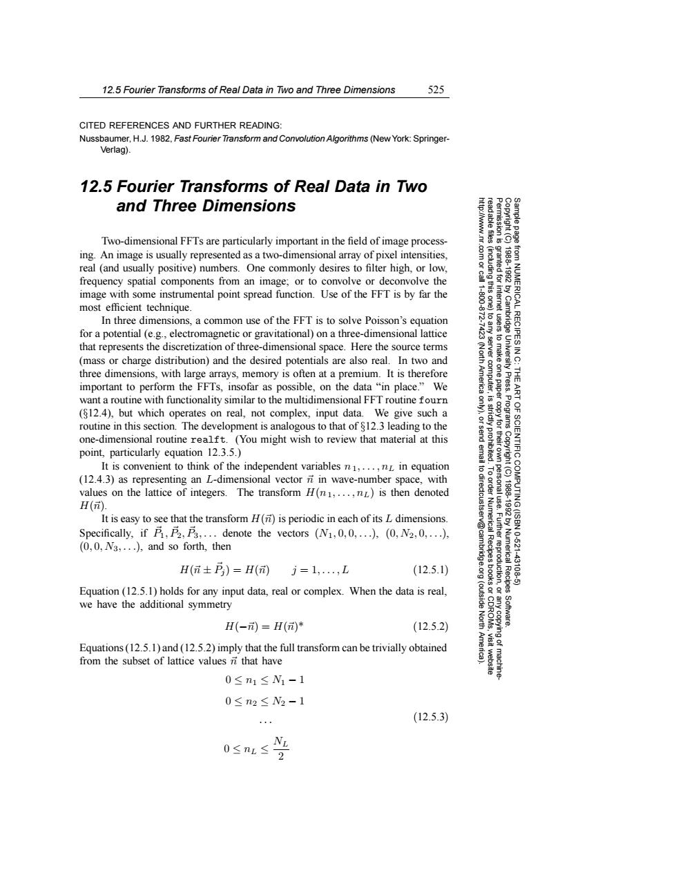
12.5 Fourier Transforms of Real Data in Two and Three Dimensions 525 CITED REFERENCES AND FURTHER READING: Nussbaumer,H.J.1982.Fast Fourier Transform and Convolution Algorithms(New York:Springer- Verlag) 12.5 Fourier Transforms of Real Data in Two and Three Dimensions Two-dimensional FFTs are particularly important in the field of image process- ing.An image is usually represented as a two-dimensional array of pixel intensities, real (and usually positive)numbers.One commonly desires to filter high,or low, frequency spatial components from an image;or to convolve or deconvolve the nted for image with some instrumental point spread function.Use of the FFT is by far the most efficient technique. In three dimensions.a common use of the FFT is to solve Poisson's equation for a potential (e.g.,electromagnetic or gravitational)on a three-dimensional lattice that represents the discretization of three-dimensional space.Here the source terms (mass or charge distribution)and the desired potentials are also real.In two and three dimensions,with large arrays,memory is often at a premium.It is therefore important to perform the FFTs,insofar as possible,on the data"in place."We 、3&ad旧日 Press. want a routine with functionality similar to the multidimensional FFT routine fourn ($12.4),but which operates on real,not complex,input data.We give such a g% 9 routine in this section.The development is analogous to that of $12.3 leading to the one-dimensional routine realft.(You might wish to review that material at this point,particularly equation 12.3.5.) OF SCIENTIFIC( It is convenient to think of the independent variables n1,...,nL in equation 61 (12.4.3)as representing an L-dimensional vector n in wave-number space,with values on the lattice of integers.The transform H(n1,...,nL)is then denoted H(). It is easy to see that the transform H(n)is periodic in each of its L dimensions. Specifically,if B,P2,P3,...denote the vectors (N1,0,0,...),(0,N2,0,...), (0,0,N3,...),and so forth,then P Numerica 10621 H(元±P)=H()j=1,,L (12.5.1) 43106 Equation(12.5.1)holds for any input data,real or complex.When the data is real, we have the additional symmetry (outside H(-)=H()* (12.5.2) North Equations(12.5.1)and(12.5.2)imply that the full transform can be trivially obtained from the subset of lattice values n that have 0≤n1≤N1-1 0≤n2≤N2-1 EE (12.5.3) L 0<nL≤212.5 Fourier Transforms of Real Data in Two and Three Dimensions 525 Permission is granted for internet users to make one paper copy for their own personal use. Further reproduction, or any copyin Copyright (C) 1988-1992 by Cambridge University Press. Programs Copyright (C) 1988-1992 by Numerical Recipes Software. Sample page from NUMERICAL RECIPES IN C: THE ART OF SCIENTIFIC COMPUTING (ISBN 0-521-43108-5) g of machine￾readable files (including this one) to any server computer, is strictly prohibited. To order Numerical Recipes books or CDROMs, visit website http://www.nr.com or call 1-800-872-7423 (North America only), or send email to directcustserv@cambridge.org (outside North America). CITED REFERENCES AND FURTHER READING: Nussbaumer, H.J. 1982, Fast Fourier Transform and Convolution Algorithms (New York: Springer￾Verlag). 12.5 Fourier Transforms of Real Data in Two and Three Dimensions Two-dimensional FFTs are particularly important in the field of image process￾ing. An image is usually represented as a two-dimensional array of pixel intensities, real (and usually positive) numbers. One commonly desires to filter high, or low, frequency spatial components from an image; or to convolve or deconvolve the image with some instrumental point spread function. Use of the FFT is by far the most efficient technique. In three dimensions, a common use of the FFT is to solve Poisson’s equation for a potential (e.g., electromagnetic or gravitational) on a three-dimensional lattice that represents the discretization of three-dimensional space. Here the source terms (mass or charge distribution) and the desired potentials are also real. In two and three dimensions, with large arrays, memory is often at a premium. It is therefore important to perform the FFTs, insofar as possible, on the data “in place.” We want a routine with functionality similar to the multidimensional FFT routine fourn (§12.4), but which operates on real, not complex, input data. We give such a routine in this section. The development is analogous to that of §12.3 leading to the one-dimensional routine realft. (You might wish to review that material at this point, particularly equation 12.3.5.) It is convenient to think of the independent variables n1,...,nL in equation (12.4.3) as representing an L-dimensional vector n in wave-number space, with values on the lattice of integers. The transform H(n1,...,nL) is then denoted H( n). It is easy to see that the transform H( n) is periodic in each of its L dimensions. Specifically, if P 1, P 2, P 3,... denote the vectors (N1, 0, 0,...), (0, N2, 0,...), (0, 0, N3,...), and so forth, then H( n ± P j ) = H( n) j = 1,...,L (12.5.1) Equation (12.5.1) holds for any input data, real or complex. When the data is real, we have the additional symmetry H(− n) = H( n)* (12.5.2) Equations (12.5.1) and (12.5.2) imply that the full transform can be trivially obtained from the subset of lattice values n that have 0 ≤ n1 ≤ N1 − 1 0 ≤ n2 ≤ N2 − 1 ··· 0 ≤ nL ≤ NL 2 (12.5.3)