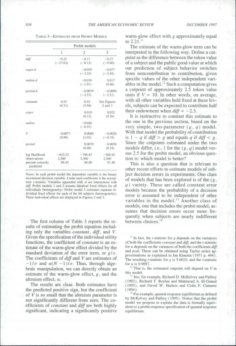
836 THE AMERICAN ECONOMIC REVIEW DECEMBER 1997 TABLE 3-ESTIMATES FROM PROBIT MODELS Probit models The estimate of the warm-glow term can be 3 interpreted in the following way.Define a cut point as the d erence between the token v at whic exper.d ←9 specific values of the other independent vari ables in the model. 9 2 pproximately els,subjects can be expected to contribute half 8% their endowment when diff= -2.5 It is instructive to contrast this estimate to the the d on te 8 is I g if diff>g and equals g it diff<g Since the under h de sus 2.5 for hit ion which model s bette This is also a question that is relevant to models of mes of the cal fied effects for al q)variety.These are calied constant error models because the probability of a decision othe etween o es of bo of the e s of -1)/o.Thus,through alge a on,we nd n this m altruism effect.a. nd Palf The results are clear.Both estimates have and Colin F.Can sign,but the coefficient (1994 tal n m as define nt fr y al resp significant,indicating a significantly positive836 THE AMERICAN ECONOMIC REVIEW DECEMBER 1997 TABLE 3^ESTIMATES FROM PROBIT MODELS diff exper.d endow.d peritid.d constant exper endow V period log likelihood observaiions perceni correctly predicled 1 -0.25 (-27,63) 0.55 (6,31) 0,0077 (0,90) -810,23 2.560 86.45 Probit models 2 -0.17 (-8.12) -0.059 (-3,23) -0.034 (-1.91) -0.0079 (-2.53) 0.52 (3.94) 0.010 (0.12) -0.046 (-0,55) 0.0089 (1,02) 0.0070 (0.46) -796,87 2,560 86,60 3 -0.27 (-9,60) -0.077 (-3.45) 0.017 (0.66) -0.0096 (-2,51) See Figures 2 and 3 0.025 (0.26) -0.0020 (-0,19) 0.0058 (0,34) -588,92 2,560 91.48 Notes: In each probil model the dependeni variable is Ihe binary inveslmenl decision variable. Under each coefficient is [he asymp￾totic /-statistic. Variables appended with .d are interactions with diff. Probit models I and 2 assume identical fixed etfecis for all individuals (homogeneity). Probit model 3 estimates separate in￾dividual fixed effects for each of the 64 subjects (heterogeneity). These individual effects are displayed in Figures 2 and 3, The first column of Table 3 reports the re￾sults of estimating the probit equation includ￾ing only the variables constant, diff, and V. Given the specification ofthe individual utility functions, the coefficient of constant is an es￾timate of the warm-glow effect divided by the standard deviation of the error term, or gla. The coefficients of diffdind V are estimates of -I/CT and a{N — l)/cr. Thus, through alge￾braic manipulation, we can directly obtain an estimate of the warm-glow effect, g, and the altruism effect, a. The results are clear. Both estimates have the predicted positive sign, but the coefficient of V is so small that the altruism parameter is not significantly different from zero. The co￾efficients of constant and diff are both highly significant, indicating a significantly positive warm-glow effect with g approximately equal to 2.21." The estimate of the warm-glow term can be interpreted in the following way. Define a cut￾point as the difference between the token value of a subject and the public good value at which our prediction of subject behavior switches from noncontribution to contribution, given specific values of the other independent vari￾ables in the model.'^ Such a computation gives a cutpoint of approximately 2,5 token value units if V = 10. In other words, on average, with all other variables held fixed at these lev￾els, subjects can be expected to contribute half their endowment when diff = —2,5. It is instructive to contrast this estimate to the one in the previous section, based on the very simple, two-parameter (g, q) model. With that model the probability of contribution is I — g if diff > g and equals q if diff < g. Since the cutpoints estimated under the two models differ, i,e., 1 for the (g, q) model ver￾sus 2,5 for the probit model, an obvious ques￾tion is: which model is better? This is also a question that is relevant to other recent efforts to estimate models of sub￾ject decision errors in experiments. One class of models that has been explored is of the (g, q) variety. These are called constant error models because the probability of a decision error is assumed to be independent of other variables in the model.'^ Another class of models, one that includes the probit model, as￾sumes that decision errors occur more fre￾quently when subjects are nearly indifferent between choices.''* '' In fact, the /-statistic for g depends on the variances of both the coefficients constant and diff. and the /-statistic for a depends on the variances of both the coefficients diff and pval. These can be obtained using Taylor series ap￾proximations as explained in Jan Kmenta (1971 p. 444). The resulting r-st£Uistic for g is 5.6010, and Che /-statistic for a is 0.9097, '- That is, the estimated cutpoint will depend on V in this model. " See, for example, Richard D, McKelvey and Palfrey (1992), Richard T, Boylan and Mahmoud A. El-Gamal (1993), and David W. Harless and Colin F, Camerer (1994), '^ For example, quantal response equilibrium as defined by McKelvey and Palfrey (1995). Notice ihat the probit model we propose to explain the data is formally equiv￾alent to a probit response specification of quanta! response equilibrium